Why Variance Can Hide a Good Strategy: A Practical Evaluation Framework

Why Variance Can Hide a Good Strategy: Overview

Variance and short samples can make even a carefully designed prediction method look like it is failing. See Funded Plays.

This overview previews the tools we will use: confidence intervals to measure estimation uncertainty, Monte Carlo and bootstrap simulation to visualize plausible performance paths, and run length diagnostics to understand how long streaks can occur by chance. These diagnostics together help set reasonable expectations and support pre-registered decision rules.

The guidance below emphasizes practical application rather than mathematical proofs. No single test proves a strategy is sound, and none guarantee future results. Instead, combine interval estimation, simulation bands, and run length thinking to make a defensible call about whether a drawdown is variance or evidence of failure.

Separating true edge from short-run noise

In practice, an estimated edge is the measured average advantage a method shows over many events. Small samples inflate uncertainty about that estimate because each additional result has a large influence on the measured average.

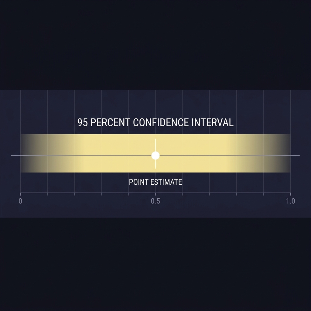
When a measured edge comes from a few dozen or a few hundred events, the confidence you can place in that edge is limited. A wide 95 percent confidence interval is a clear signal of imprecision and can indicate that the observed advantage is not statistically persuasive for the sample at hand, which is why interval interpretation matters early in testing NCBI Bookshelf guidance on confidence intervals.

Event frequency also matters. Low-frequency sports or niche markets will naturally require more calendar time to reach the same sample sizes as higher-frequency markets, and that should shape expectations about how long a test must run before conclusions are drawn.

How confidence intervals reveal uncertainty

A 95 percent confidence interval around an estimated edge describes a range that, under repeated sampling, would contain the true effect about 95 percent of the time. For a practitioner this means that a wide interval reflects substantial uncertainty about the underlying advantage Cochrane Handbook guidance on interpreting confidence intervals. See also PubMed article on confidence intervals.

Correct interpretation is critical. If the interval includes zero, the observed edge is not statistically proven for that sample, even if the point estimate is positive. That does not mean the strategy is worthless, only that available data are inconclusive.

For practical decisions, treat intervals that are too wide to exclude trivial outcomes as inconclusive and either continue collecting data or tighten your minimum effect size before acting.

Using Monte Carlo and bootstrapping to visualize dispersion

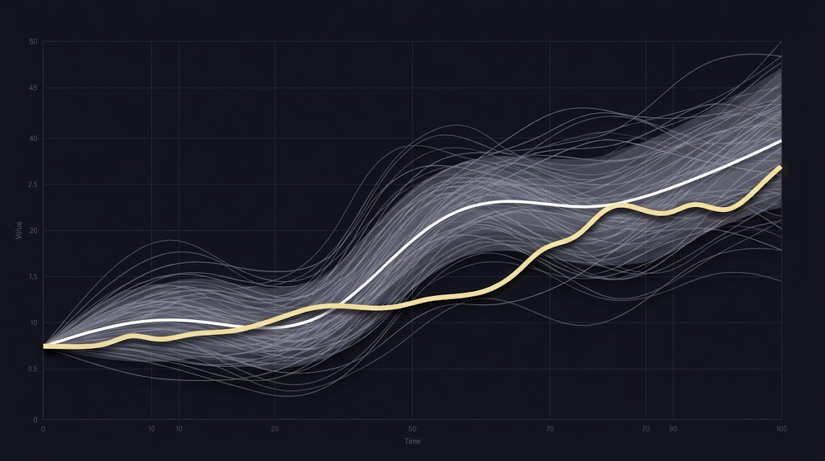
Monte Carlo simulation lets you generate many plausible performance paths consistent with assumed parameters for mean, variance, and other features of returns. Running thousands of simulated paths creates an envelope of typical outcomes and shows how often a positive-EV process produces temporary underperformance Encyclopaedia Britannica on the Monte Carlo method, and a practical guide is available at StrategyQuant.

When distributional assumptions are questionable, bootstrapping provides a data driven alternative by resampling observed returns to produce empirical performance bands without strong parametric assumptions. Both approaches help turn a single observed equity path into a calibrated question: is this drawdown unusual given the assumed or observed parameters?

Simulations are particularly valuable because they make explicit how often a strategy with modest edge is expected to experience long losing stretches. Visualizing those paths reduces the tendency to treat a single string of losses as definitive evidence of structural failure.

Average run length and why long streaks happen by chance

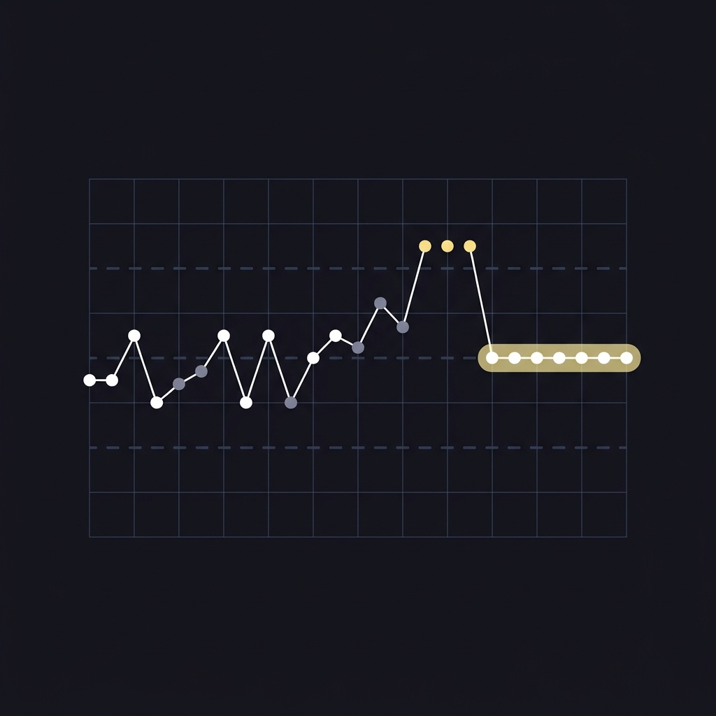
Average run length, or ARL, is a control-chart concept that predicts how often a monitoring rule will trigger by chance under a stable process. ARL theory explains why long streaks and apparent false alarms occur even when the underlying process is unchanged NIST e-Handbook on average run length.

Funded Plays Challenges

View FundedPlays Challenges

Using ARL to choose monitoring thresholds helps you balance sensitivity and false alarm rate. A very sensitive stop rule will catch true failures faster but also trigger more false alarms. Conversely, an insensitive rule may allow real degradation to continue too long. ARL calculations let you quantify that tradeoff before you go live.

Detecting overfitting and multiple testing risks

Backtest overfitting happens when a method is tuned to past noise rather than to an underlying predictive signal. The more parameters or filters you try, the greater the chance of finding a combination that looks strong by luck rather than because it will persist out of sample.

Reality-check style tests and deflated Sharpe diagnostics are corrective approaches that adjust for the multiple testing problem and reduce the risk of promoting a spurious strategy to live testing Notices of the AMS discussion on backtest overfitting.

Preserve a genuine out of sample holdback and pre-register hypotheses where feasible. Treat any parameter change after seeing results as a new hypothesis that must be evaluated with fresh data rather than retroactively rationalized.

Combining confidence intervals, simulation, and run length diagnostics

No single test is decisive. Confidence intervals quantify estimation uncertainty. Simulations produce expected envelopes for equity paths. Run length diagnostics show how often monitoring rules will flag apparent problems by chance. Layering these methods makes a more defensible judgment.

Overlay your observed equity path on simulation envelopes and check whether the path regularly falls outside typical percentiles. If the path remains within plausible bands and ARL expectations, the drawdown is more likely variance than structural failure Encyclopaedia Britannica on the Monte Carlo method.

Use interval checks, simulation bands, and ARL together. For example, require that a 95 percent confidence interval excludes a minimum pre-registered effect size, the observed path not cross the 5th percentile of simulated outcomes, and run lengths not exceed an ARL-based alarm rate before declaring structural failure.

A practical evaluation framework: pre-registration, thresholds, and sample rules

Pre-register testing rules and thresholds before live testing. That should include a minimum sample size, a minimum detectable effect size, the maximum tolerable drawdown, and the monitoring cadence. Pre-registration reduces data snooping and makes later decisions defensible. Learn more in how Funded Plays evaluations work.

Choose minimum sample sizes based on desired interval width and event frequency. Wider acceptable confidence intervals require larger samples to detect the same effect. Use the interval formulas to plan how many events are needed to estimate an effect with the precision you require NCBI Bookshelf guidance on confidence intervals.

Define drawdown tolerance relative to typical simulated outcomes. For example, set a rule that a pause or structural review is triggered only if the observed drawdown exceeds the 95th percentile of simulated worst drawdowns for the pre-registered horizon.

Decision criteria: when to keep testing and when to stop

Combine criteria rather than relying on a single trigger. A defensible stopping rule can require that the confidence interval for the edge crosses zero, the observed path breaches a low simulation percentile, and observed run lengths exceed ARL-based thresholds before pausing the strategy.

This composite approach balances Type I and Type II errors. Requiring multiple signals reduces false positives at the cost of slower detection of genuine degradation. For small samples, err on the side of continued testing rather than abrupt termination, but document every decision and its rationale NIST discussion on run length and monitoring.

If you change parameters, treat the modified method as a new hypothesis and re-enter the pre-registered testing process rather than folding past results into the revised model.

Typical mistakes and pitfalls to avoid

Common errors include overreacting to short drawdowns, ignoring confidence interval width, failing to correct for multiple tests, and altering rules after seeing results. Each of these inflates the risk of discarding a good strategy or persisting with a poor one.

Parameter tinkering after the fact is a particularly dangerous habit because it effectively multiplies the number of tests you have run. Use reality-check style corrections to account for that risk and keep a documented log of hypothesis tests and changes SSRN working paper on overfitting risk.

Practical sports prediction scenarios

Scenario one, low frequency events: a niche sports market that offers 100 decisions a year will accumulate evidence slowly. Expect wide confidence intervals for many months and use simulation to see how often long losing stretches appear by chance under a modest positive edge Encyclopaedia Britannica on simulation methods. Another introduction is available at Lumivero.

Scenario two, high variance leagues: a high variance league with frequent upsets may produce noisy short-term records. Simulations based on observed variance help set realistic drawdown tolerances and show that a several month losing run can be consistent with a positive long-term edge.

In both scenarios, pre-registered minimum effect sizes and sample sizes should reflect event frequency and variance. This reduces the chance that short-term noise leads to premature stopping or unwarranted confidence.

Monitoring live performance and diagnosing drawdowns

Create an operational monitoring checklist that updates confidence intervals on a defined cadence, overlays observed equity on simulation envelopes, and tracks run length statistics against ARL-based alert thresholds. Regular automated reports make decisions reproducible and less emotional. See our blog for monitoring cadence and reporting examples.

When a drawdown exceeds a pre-registered threshold, follow a documented escalation path: pause new allocation, run a fresh set of simulations using the latest data, examine for rule changes or data integrity issues, and escalate to a review panel if multiple diagnostics indicate structural concerns NIST guidance on monitoring and false alarms.

Keep concise records of every review and decision. Documentation reduces hindsight bias and provides the evidence trail needed when evaluating whether a change was warranted.

Putting it together: a checklist for researchers and competitors

Pre-test checklist items should include pre-registration of hypotheses, minimum sample size, minimum effect size, planned simulation approach, ARL-based monitoring thresholds, and a specified reporting cadence. These items make tests reproducible and decisions traceable.

Live monitoring checklist items should include updated confidence intervals, simulation envelope checks at the chosen percentiles, run length alerts, documentation of any parameter changes, and a quarterly calibration review to ensure thresholds remain appropriate for event frequency and variance NCBI Bookshelf guidance on interval estimation.

Conclusion: patience, discipline, and next steps

Variance can mask a good strategy, but it can also hide structural problems. The practical response is consistent procedures: pre-register, run simulation and bootstraps, apply ARL thinking, and document every decision so that you can distinguish noise from true failure with evidence.

Immediate actions for practitioners: pre-register your testing rules, estimate the sample size needed to reach useful interval width, build a simulation plan, and adopt ARL-based monitoring thresholds. None of these steps guarantees success, but together they reduce mistakes and support disciplined, transparent evaluation.