Which Sports Statistics Are Most Predictive, and How to Use Them

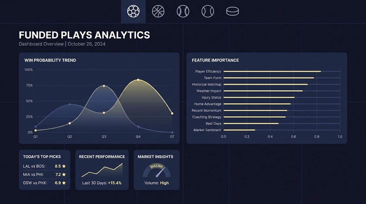
Introduction: why predictive statistics matter for forecasting

What we mean by predictive, Which Sports Statistics Are Most Predictive

When we ask which statistics actually predict future results we mean measures that consistently improve out-of-sample forecasts rather than simply summarizing what happened in a single game. Predictive features are those that add information a model can use to make more accurate probabilistic forecasts over time.

Descriptive statistics, like a box score total, summarize past events. Predictive statistics aim to capture underlying processes that persist into the future, such as shot quality or context-adjusted play value. Establishing a statistic as predictive requires testing on data that were not used to build the feature or model to avoid overfitting.

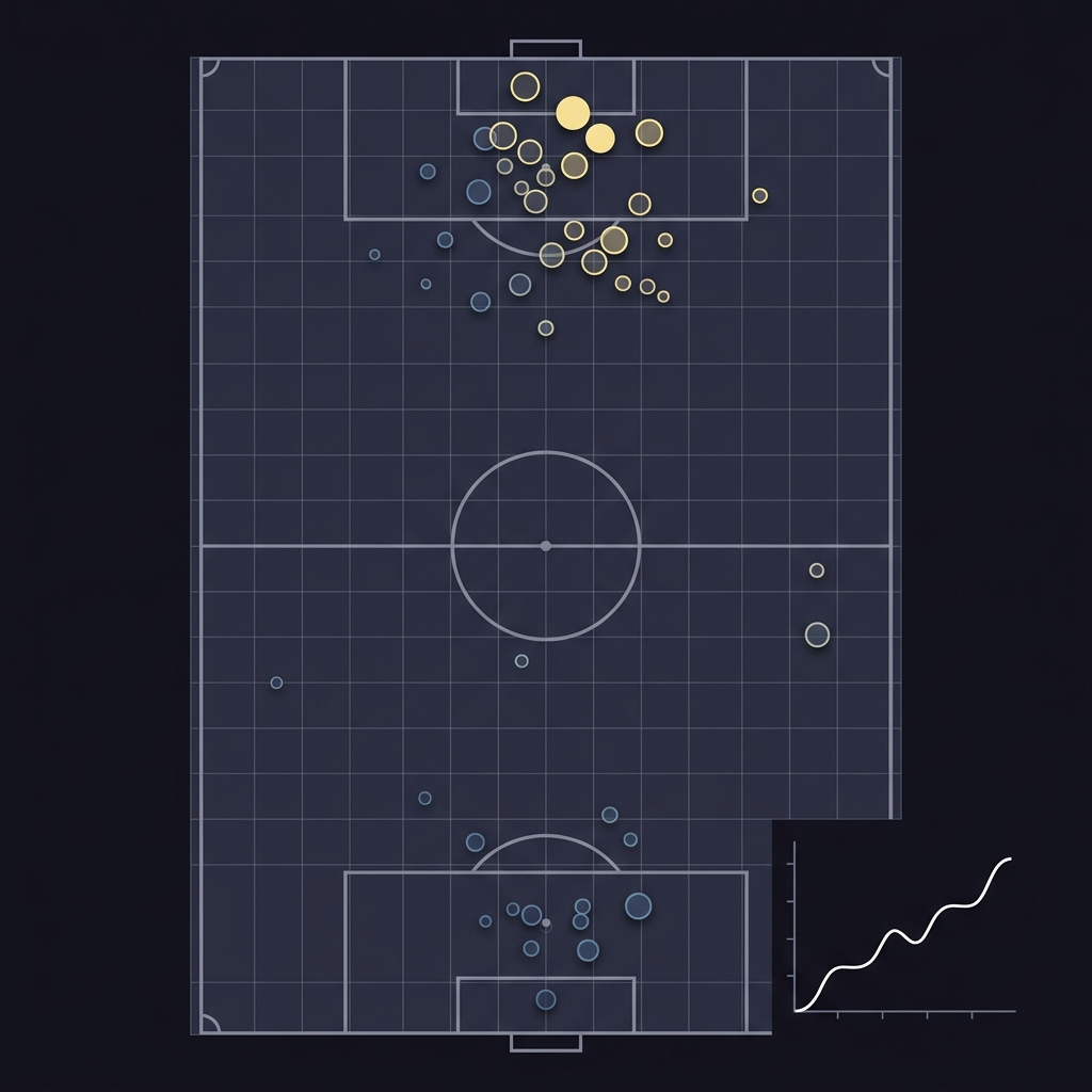
Prediction focuses on forward-looking performance and demands validation routines that mimic the forecasting task. Good practice uses time-aware holdouts and checks for stability across seasons. A feature that helps explain variance in a single season may fail to generalize when evaluated properly, so the distinction between description and prediction is central to reliable sports analytics work.

How prediction differs from description

How to evaluate predictive power: scoring rules and validation

Proper scoring rules explained

Two widely recommended measures for probabilistic forecasts are the Brier score and log loss, which reward well-calibrated probability estimates and penalize overconfidence; these proper scoring rules are foundational for model comparison and calibration checks Journal of the American Statistical Association article on scoring rules.

Calibration and discrimination are complementary: calibration checks whether predicted probabilities match observed frequencies, while discrimination measures how well the model separates outcomes. Both should be reported because a model can be well discriminating but poorly calibrated, or vice versa.

Cross validation and test splits that matter

For time-series sporting data, use holdout periods that follow the training window to avoid lookahead bias, and prefer rolling backtests when seasonality or roster turnover matters. Cross validation that ignores temporal structure can give overly optimistic results.

When reporting performance, present both aggregate scores and season-level summaries so readers can see whether strong performance is concentrated in a short window or stable across multiple seasons.

Core methodological framework: feature importance, regularization and backtesting

Why regularization helps rank features

Regularized regression reduces variance by shrinking weak coefficients toward zero, which helps separate genuinely predictive features from correlated noise. Using penalty-based methods like elastic net offers a principled way to select features while controlling complexity.

Tree models and permutation importance

Tree-based models provide alternative importance measures, such as permutation importance, that assess how much predictive error increases when a feature is shuffled; these methods complement coefficient-based rankings and can capture nonlinear relationships.

Backtesting protocols to avoid false discoveries

Rankings are only useful when validated with cross-validated backtesting across multiple seasons and sample splits to test stability and avoid false discoveries. Routine out-of-sample evaluation is a core component of a defensible ranking workflow systematic review on machine learning for sports prediction.

Be careful to include preprocessing steps inside each cross-validation fold and to avoid using future-derived features that leak information. A clear pipeline that mirrors production scoring is essential for honest evaluation.

Soccer: expected goals and why xG outperforms raw goals in short samples

What xG measures and how it is computed

Expected goals, or xG, assigns a probability to each shot based on contextual features such as shot location, type of assist and situation, estimating the likelihood that a shot becomes a goal. Because xG captures shot quality rather than binary outcomes, it tends to be less noisy in the short term.

Empirical practitioner work shows that xG often tracks underlying team quality better than raw goals in short samples, which makes it useful for predicting near-term performance and correcting for random goal variance The Analyst explainer on expected goals. See practitioner analysis at StatsBomb.

Limitations include differences between providers and sensitivity to the underlying event data. For robust forecasting, treat xG as a core input but validate provider choices and consider aggregating over multiple matches to reduce provider noise.

American football (NFL): Expected Points Added and context-adjusted efficiency

What EPA captures that yards do not

Expected Points Added, or EPA, measures how a play changes a team's expected scoreboard outcome by accounting for down, distance and game state. Two plays with the same yardage can have very different EPA when the context is included.

How to use EPA in team-level prediction

EPA-based efficiency metrics correlate more strongly with winning than raw yardage totals because they value situational importance and scoring context; this makes EPA a preferred basis for team-level forecasting when play-by-play data quality is sufficient journal article on reproducible player evaluation in football.

When building models, adjust EPA measures for opponent strength and sequencing and examine whether aggregated per-play EPA or drive-level EPA better fits the forecast horizon you care about.

Basketball (NBA): the Four Factors and why shooting efficiency and turnovers matter most

Breakdown of the Four Factors

The Four Factors are shooting efficiency, turnover rate, rebounding and free-throw performance. They provide a parsimonious framework to explain scoring and defense, and they are commonly used as inputs to predictive models of team outcomes.

Evidence for eFG% and turnover rate as top predictors

Across studies, effective field goal percentage and turnover rate typically have the strongest relationship with point differential and wins, making them central to models that forecast team success in the NBA study on factors influencing NBA team success.

Rebounding and free-throw rate play supporting roles and can become more important in specific matchups or on teams with elite rebounders or foul-drawing players.

Baseball (MLB): wOBA, xwOBA and modeling run creation

Why composite run-creation metrics outperform basic averages

wOBA weights on-base outcomes by their run value to produce a single-number measure of offensive contribution that outperforms simple averages like batting average for forecasting run production.

Using expected variants like xwOBA for forward-looking models

Expected versions such as xwOBA aim to filter out luck from observed outcomes by modeling the quality of contact and context, which can improve the signal for future run scoring when combined with park and lineup adjustments FanGraphs library on wOBA.

Practical limits include park effects and batting order composition; incorporate those adjustments explicitly when you use wOBA or xwOBA in predictive models.

Cross-sport comparison: how predictive strength differs by metric and sport

What makes a metric transferable across sports

Transferability depends on whether a metric captures a sport-invariant concept such as efficiency per opportunity, versus a sport-specific context like pitch sequencing or set pieces. Rate statistics that normalize by opportunity are more likely to generalize than raw counting stats.

When to prefer rate stats over counting stats

For prediction, rate statistics are often more stable because they adjust for usage and playing time, which reduces variance in small samples. Use rate stats where sample size is limited and counting stats where long-term accumulation is acceptable systematic review on machine learning for sports prediction.

Always align the metric choice with sample size and season length; what works for a sport with many events per season may not translate to one with few games.

Decision criteria: choosing metrics for your forecasting objective

Define your objective and forecast horizon

Start by clarifying whether you need a single-game probability, a season projection or a player-level ranking. Forecast horizon affects which metrics are useful: short horizons favor in-game efficiency measures, longer horizons benefit from stabilized rate metrics and aging adjustments.

Align features to the prediction task

Use a simple checklist when selecting features: predictive stability across seasons, interpretability for troubleshooting, availability of data, and alignment with the forecast horizon. Validate chosen features with holdout tests before production deployment Journal of the American Statistical Association article on scoring rules.

Prefer a small set of robust, interpretable features over a large unstable set that risks overfitting. When in doubt, test both and compare out-of-sample performance.

Typical mistakes and pitfalls when ranking predictive statistics

Data leakage and lookahead bias

A common error is leaking future information into training features, which produces unrealistically optimistic in-sample results. Time-aware splits and careful pipeline design prevent this form of bias.

Misreading correlations as predictive power

Correlation in-sample is not proof of predictive skill. Small-sample correlations can be driven by variance or confounding; validate relationships across multiple seasons and with out-of-sample testing to gain confidence systematic review on machine learning for sports prediction.

Also watch for unadjusted counting stats that fail to account for opportunity; a high raw total may reflect volume rather than higher per-opportunity quality.

Practical example: building a simple probabilistic model for match outcomes

Selecting features and preprocessing

Begin by choosing a small, interpretable feature set aligned with your sport and horizon. For soccer a compact set might include team xG per 90, recent form as a rolling average, and an opponent-adjusted defensive xG metric. Normalize per-90 or per-possession as appropriate and impute missing values with simple domain-aware rules.

Evaluating with proper scoring rules

Train a logistic or regularized probabilistic model and evaluate on a time-based holdout using Brier score or log loss. Plot calibration and, if necessary, apply simple recalibration techniques to align predicted probabilities with observed frequencies Journal of the American Statistical Association article on scoring rules.

Document the training pipeline and include preprocessing inside cross-validation folds. Report both aggregate scores and season-level performance to understand consistency. If the model is miscalibrated, use simple isotonic or logistic recalibration applied only on a validation fold.

Data, features and tools: what to collect and basic preprocessing steps

Essential data fields and quality checks

Collect play-by-play entries when available, shot coordinates for soccer and basketball, box score statistics and timestamps. Check for missing timestamps, inconsistent event labeling and duplicated entries as part of basic quality control.

Simple feature engineering examples

Create rolling averages for recent performance, opponent-adjusted metrics that weight by opponent strength, and pace or opportunity-normalized rates. Keep engineered features transparent so you can trace performance back to data inputs systematic review on machine learning for sports prediction.

Store intermediate datasets and random seeds so experiments are reproducible and easier to audit when results change.

Skill-focused platforms can structure evaluation challenges where participants use virtual funded accounts and defined objectives to demonstrate forecasting stability rather than wagering real funds. Link to details on evaluation challenges.

Funded Plays Challenges page

Review the challenge checklist

Success in structured challenges is demonstrated by consistent, rule-compliant forecasting and steady progress across evaluation steps. Platforms that use virtual bankrolls and explicit drawdown rules reward measured, repeatable skill rather than single-event wins. For more context see structured challenge posts.

Participants should align their feature choices to the rules of the challenge and validate their approach with backtests that mimic the challenge sequence before entering live evaluation. See the site homepage for general information Funded Plays.

Conclusion: practical takeaways and next steps for readers

A short checklist to apply today

Use proper scoring rules for probabilistic forecasts, prefer rate or context-adjusted metrics for small samples, validate rankings with cross-validated backtesting, and monitor calibration over time. These steps reduce the chance of trusting spurious relationships.

Further reading and validation next steps

Experiment incrementally: start with a few robust, interpretable features, evaluate on time-aware holdouts, then add complexity only when it improves out-of-sample scores. Track results over multiple seasons to confirm stability before relying on any single metric for decision making. For additional posts see our blog.

References

- https://www.tandfonline.com/doi/abs/10.1198/016214506000001437
- https://www.frontiersin.org/articles/10.3389/fspor.2023.000000/full
- https://theanalyst.com/na/2024/02/what-are-expected-goals-xg-explained/
- https://doi.org/10.1515/jqas-2018-0100
- https://content.iospress.com/articles/journal-of-sports-analytics/jsa210
- https://www.fangraphs.com/library/offense/woba/
- https://www.fundedplays.com/challenges
- https://pmc.ncbi.nlm.nih.gov/articles/PMC10075453/
- https://blogarchive.statsbomb.com/articles/soccer/the-dual-life-of-expected-goals-part-1/
- https://www.hudl.com/blog/expected-goals-xg-explained
- https://www.fundedplays.com
- https://www.fundedplays.com/blogs
- https://www.fundedplays.com/blogs/how-fundedplays-evaluations-work