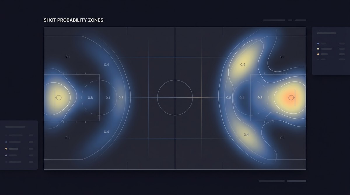
Using Shot Quality Instead of Shot Count

Using Shot Quality Instead of Shot Count: What it Means

Using Shot Quality Instead of Shot Count is a simple shift in emphasis: move from counting every attempt the same way to weighting attempts by how likely they were to score. This change recognises that a low, blocked long-range strike and a close-range header with an open goal are not equal events for forecasting or evaluation.

Start by separating two plain concepts. "Shot count" is the raw tally of attempts a team or player makes in a match. It is easy to measure and easy to report. "Shot quality" expresses the chance each attempt had of producing a goal, so several low-probability shots add less weight than a few high-probability chances.

One helpful analogy: think of shot count like counting the number of seeds in a basket and shot quality like measuring the weight and ripeness of each piece of fruit. The count tells you volume, the quality tells you likely yield.

Definitions: shot quality, shot count, and context

Shot count remains useful when you want to measure offensive activity or pressure in bulk. It is an unbiased, transparent number that is hard to misreport. Shot quality, by contrast, uses context to estimate scoring probability. Common proxies include expected goals, location-based probability tables, and post-shot measures that factor in shot placement.

Why the shift matters for prediction and evaluation

When prediction accuracy is the goal, weighting by quality reduces noise from long sequences of low-probability attempts and surfaces the attempts most likely to change the scoreboard. That makes models better aligned with what actually determines goals and with the short-term outcomes many forecasters care about.

As you read the rest of this article, notice how the language moves from descriptive to operational: the focus is on how to apply quality metrics in real workflows, not just on why they matter.

Why Using Shot Quality Instead of Shot Count Improves Analysis

Shot-quality metrics formalise intuition: not all shots are created equal. A small set of high-probability chances can explain a match result more reliably than a larger set of speculative attempts. For forecasting and model calibration, this reduces measurement noise and helps models learn signals tied to scoring rather than to volume alone.

In predictive work, noisy inputs create unstable models. By replacing raw counts with quality-weighted totals, you guide a model to prioritise features that map to scoring probability. This matters in short-term forecasts, live prediction adjustments, and when evaluating a player or tactic over a small number of games.

For handicappers and users on skill-based prediction platforms, emphasising quality helps separate luck-driven volume from repeatable performance. A player who consistently produces high-quality chances demonstrates a repeatable process, whereas consistent high volume with low average quality often reflects noise or a risk-seeking approach.

As a rule of thumb, use quality metrics when the question is about scoring probability or model calibration. Keep counts when you want a raw measure of activity, such as press intensity or attempts per minute.

Core Metrics and Models for Assessing Shot Quality

Shot-quality metrics give you different views on the same underlying idea. Expected goals, or xG, estimates the probability a shot becomes a goal based on features such as location and assist type. Post-shot xG refines that by accounting for where the ball actually went and how likely a goalkeeper could save it. Big-chance classification isolates the subset of attempts that carry especially high probability.

Funded Plays Challenges

View Funded Plays Challenges

Simple shot maps show raw locations and can be overlaid with a location-based probability table to create a fast proxy xG. Full xG models often add assist type, body part, phase of play, defensive proximity, and goalkeeper position for better calibration. Choose the level of detail that fits your data and resources.

Common shot-quality metrics and what they measure

Expected goals (xG): a probability estimate per shot that aggregates to an expected goals total for a match or player.

Post-shot xG: evaluates the actual placement and trajectory to refine the scoring probability after the shot is taken.

Big-chance indicators: a simplified flag to mark attempts that meet a high-probability threshold; useful for scouting and concise reports.

Model inputs: location, assist type, body part, phase of play

Standard inputs include shot location, assist type (through ball, cross, cutback), body part (head, foot), and whether the chance came from open play or a set piece. Defensive pressure and goalkeeper positioning are valuable when available.

Advanced variants: post-shot xG and shot-creation metrics

Shot-creation metrics track the sequence that produced the shot, useful when you want to reward build-up skill rather than raw finishing luck. Post-shot xG helps evaluate finishing quality and goalkeeper effect separately from chance creation.

How to Transition from Shot Count to Shot Quality in Practice

Start small. The easiest first step is to build a location-based probability table using publicly available event data and apply it to past matches. That gives you a consistent proxy for xG and a baseline to compare against raw shot counts.

Next, compute a shot-quality total for each match or player by summing the per-shot probabilities. Compare the new quality totals to previous count-based summaries to see where conclusions change.

Integrate these totals into your dashboards and scouting notes. Replace a count column with both count and quality columns during a transition period so stakeholders can see the difference without losing familiar metrics. When model performance improves consistently, phase out the reliance on counts in predictive features.

Be pragmatic about data quality: a robust xG model requires clean event data. If you lack detailed inputs like defensive pressure, a simple location-plus-assist-type proxy will still outperform raw counts for many short-term forecasting tasks.

Data sources and simple first steps

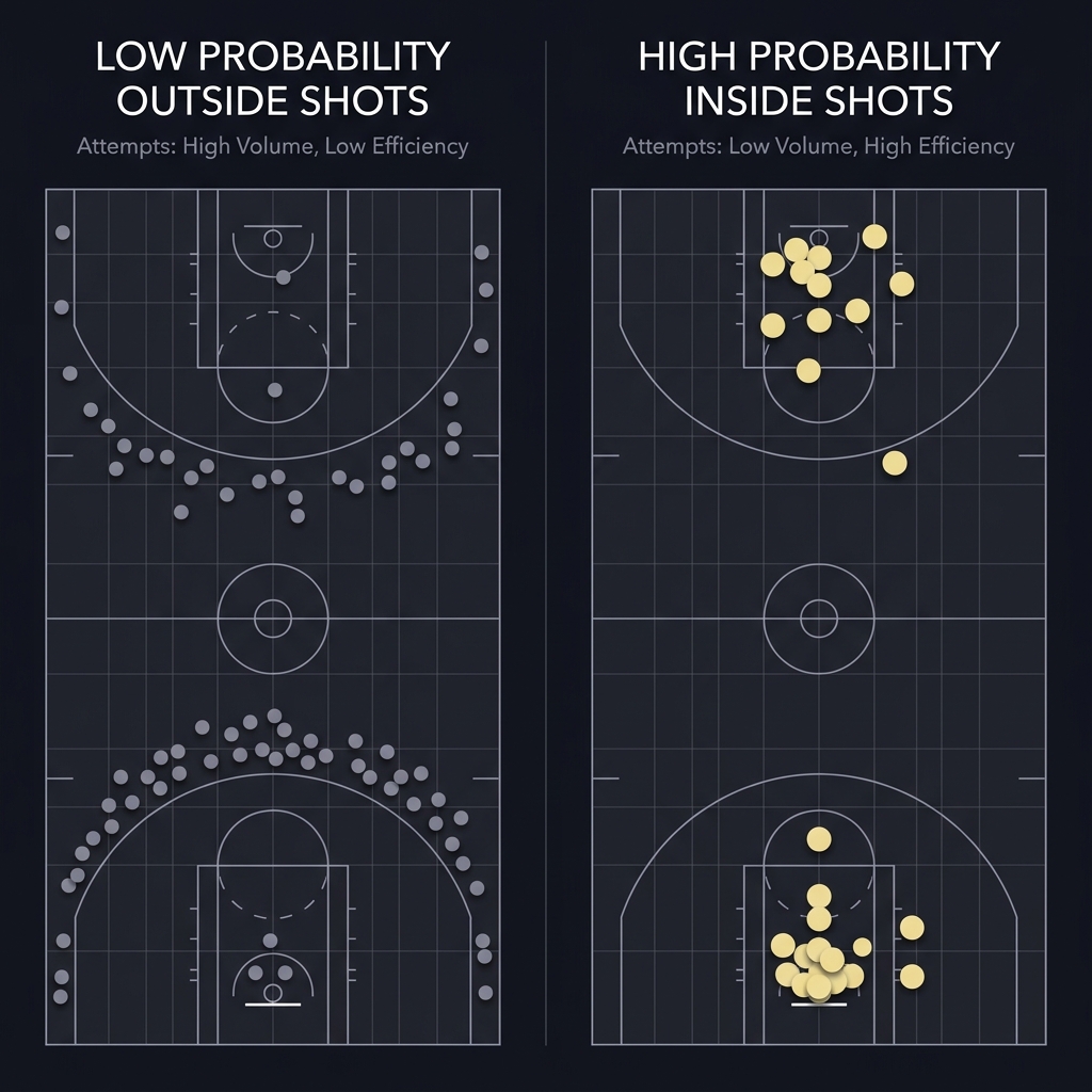
Public event feeds and match logs provide shot location and basic context. Use these to create a reproducible pipeline that tags each shot with a probability and stores both raw and weighted summaries for testing.

Building or adopting an xG proxy

A location-only table can be built from your historical data or adopted as a simple lookup. As you gather more inputs, iterate to add assist type and body part. Keep versioned models so you can roll back if a new input reduces out-of-sample performance.

Integrating shot-quality into existing workflows

When integrating, maintain both views: quality for decision-making and count for context. Update dashboards to visualise both the total xG and the distribution of shot probabilities so scouts and analysts can see whether scoring chances are clustered or dispersed.

Decision Criteria: When Shot Quality Matters More Than Volume

Decide on metric emphasis by question type. For match-level forecasting, in-play decisions, or short evaluation windows, quality is typically more informative because it ties closely to the immediate probability of goals. For season-level workload analysis or measuring sustained attacking intent, counts retain value.

Use simple decision rules. If your primary objective is to estimate scoring probability or to calibrate a predictive model, prioritise shot-quality metrics. If your aim is to measure time-on-ball, sustained pressure, or total attacking attempts across a long sample, include counts as a complementary measure.

Watch sample size. Very small samples make both counts and quality estimates unstable, but quality metrics can overfit if a model tries to explain fine-grained variance from limited data. Implement minimum sample thresholds and aggregate appropriately before making strong claims.

Match-level vs season-level uses

Match-level: prefer quality for immediate forecasting and tactical adjustments. Season-level: combine both to track trends and workload.

Types of questions best answered by quality metrics

Questions about expected goals, the likelihood a lineup will score in the next 30 minutes, or which player creates repeatable high-probability chances are best served by quality measures.

When to still use shot counts

Counts are useful for raw volume, measuring pressure, and describing a team's approach. Use counts alongside quality to avoid missing signals such as sustained low-quality pressure or fatigue-driven volume changes.

Common Mistakes and How to Avoid Them

Misreading small samples is the most frequent error. Analysts often treat a handful of matches as decisive evidence. Avoid this by setting clear aggregation rules or by reporting confidence intervals around quality estimates.

Confusing model outputs with guarantees is another pitfall. Treat xG and other probabilities as forecasts, not promises. Communicate uncertainty and avoid definitive language when sharing results with decision makers.

Over-relying on a single metric reduces robustness. Combine quality with complementary measures such as shot-creation chains, finishing indicators, and goalkeeper performance to form a more complete picture.

Misreading small samples

If a player posts a high mean quality over three games, consider a larger window before concluding it represents a true step change. Use moving averages and rolling windows to stabilise estimates.

Confusing model outputs with guarantees

Remember that probabilistic outputs can be wrong frequently in the short run. Use calibration tests and emphasize that outcomes are stochastic.

Over-relying on a single metric

Pair quality metrics with tactical context and qualitative scouting to avoid blind spots such as match-up effects or referee influence.

Practical Examples and Scenarios

Case A: Evaluating a striker over four matches. Suppose two strikers each have seven shots in four matches. Player A’s shots cluster inside the box on the penalty spot, while Player B’s attempts are mostly long-range. Summing per-shot probabilities will usually favour Player A by indicating a higher expected goals total even though the counts are equal. That difference is actionable for selection or substitution decisions.

Case B: Adjusting a model for away versus home shot quality. If a model shows that away matches produce fewer high-quality chances on average, include a venue adjustment to avoid overstating away-team finishing potential. The adjustment can be a simple scaling factor applied to per-shot probabilities or a feature in your predictive model.

Case C: Using shot-quality to inform in-play or short-term forecasts. In live forecasting, a sudden shift from low-quality long shots to sustained box entries should update short-term scoring probability more than a rise in overall shot count. Use rolling quality sums for the last 10 to 20 minutes to inform in-play estimates.

Case A: Evaluating a striker over four matches

Walk through the player comparison, showing expected goals totals and how those weights change selection thinking. Emphasise that quality points to repeatable processes rather than single-match luck.

Case B: Adjusting a model for away versus home shot quality

Explain a simple venue adjustment and how to validate it on an out-of-sample season to ensure it improves predictive performance without introducing bias.

Case C: Using shot-quality to inform in-play or short-term forecasts

Offer a short tip: use a short rolling window for quality and test live-calibration on historical matches to tune responsiveness.

Putting it Together: Checklist, Next Steps, and Caveats

Quick implementation checklist: collect event data and shot locations, build a location-based probability table, compute per-shot probabilities and sum them to create match and player xG totals, compare these to count-based summaries, update dashboards, and validate model impact using out-of-sample testing.

Monitor models continuously. Track calibration metrics, average error on short windows, and whether quality-weighted features improve decision outcomes. If performance degrades, roll back to the prior model version and investigate which input caused the issue.

Responsible interpretation is essential. No metric guarantees outcomes. Quality metrics are probabilistic tools that should be used with clear uncertainty communication and in combination with domain knowledge.

How to monitor and iterate

Use versioning for models and data, run regular calibration checks, and maintain a validation window that is separate from your training period. Keep a changelog of updates so you can connect model shifts to feature or data changes.

Responsible use and communicating uncertainty

When presenting results, provide context: describe sample size, outline what inputs the quality metric uses, and state the limits of your data. This reduces misinterpretation and supports better decisions.