Using Returning Production in Preseason Analysis: A Practical Guide

Using Returning Production in Preseason Analysis: What it is and why it matters

Using Returning Production in Preseason Analysis starts with a clear, operational definition: returning production measures the share of a team’s prior-season output that is attributable to players who remain available on the current roster, calculated from player-level counting stats rather than a simple starter flag.

That difference matters because a binary returning-starters indicator treats all starters the same, while returning-production shares reflect the actual volume of yards, targets, snaps, tackles and other contributions that carry predictive information into a new season. Evidence from squad continuity research shows that keeping more production together is associated with better team outcomes, which explains why modern preseason models favor player-level shares over starter counts in their inputs Journal of Sports Analytics study on squad continuity.

Prominent model frameworks explicitly blend returning production with recent performance and recruiting rather than relying only on who started last year. That pragmatic combination helps balance stability and recency when moving from raw counts to preseason ratings, and it is a common design in widely used college football rankings.

In short, using returning production gives modelers a continuous, measurable input that captures how much of a team’s capability returns from year to year, which improves interpretability and often enhances predictive accuracy when compared with crude starter counts.

Key components of returning production: which player stats to track

Offensive metrics: yards, targets, snaps, quarterback contributions

To compute returning shares on offense, practitioners prioritize player-level counting stats such as total offensive yards, passing yards by the quarterback, rushing and receiving yards for skill players, targets for receivers, and offensive snaps to capture involvement. These stats let you see which players accounted for volume and therefore how much offensive capability remains on the roster.

For example, tracking targets and receiving yards separates a returning backup who saw few targets from a returning lead receiver whose volume drives both production and matchups; similarly, counting offensive snaps gives a better picture of role continuity than a starter label alone.

Defensive metrics: tackles, interceptions, defensive snaps

Defensive returning-production measures typically use tackles, tackles for loss, interceptions and defensive snaps to identify experience and playmaking that will likely carry over. Defensive playmaking and experience often have outsized value for preseason assessments because lineups and assignments carry institutional knowledge that helps cohesion.

Special teams and role players should not be ignored, especially in tight games where returns in punt and kick returns or field-goal kicking can swing outcomes; include return yards and special-teams snaps where data availability allows.

Many of these player-level counting stats are available from public sources, though they may require minimal cleaning and reconciliation to handle inconsistent player naming or split roles.

Using Returning Production in Preseason Analysis: data sources and reproducible pipelines

Public sources: CollegeFootballData API and Sports-Reference

Two public, reproducible sources are practical starting points: the CollegeFootballData API for programmatic access to player-season records and Sports-Reference for season and player pages that provide full counting stats and historical context CollegeFootballData API documentation. The API root is https://api.collegefootballdata.com/, and alternative commercial feeds include SportsDataIO's NCAA API docs.

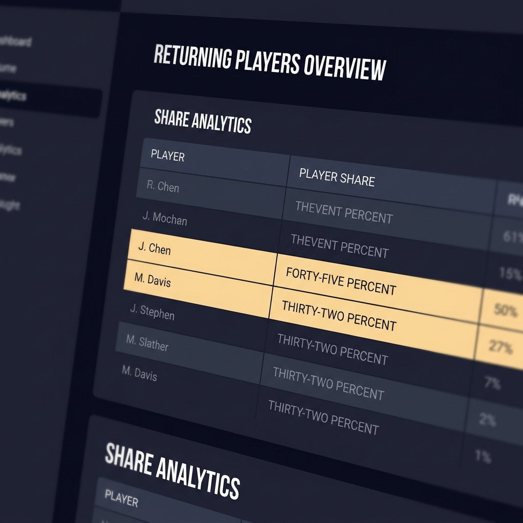
Sports-Reference’s season and player pages are also commonly used to validate or fill gaps in programmatic pulls, since they provide human-readable season summaries and player stat tables that are easy to cross-check against API extracts Sports-Reference 2024 season summary and player stats.

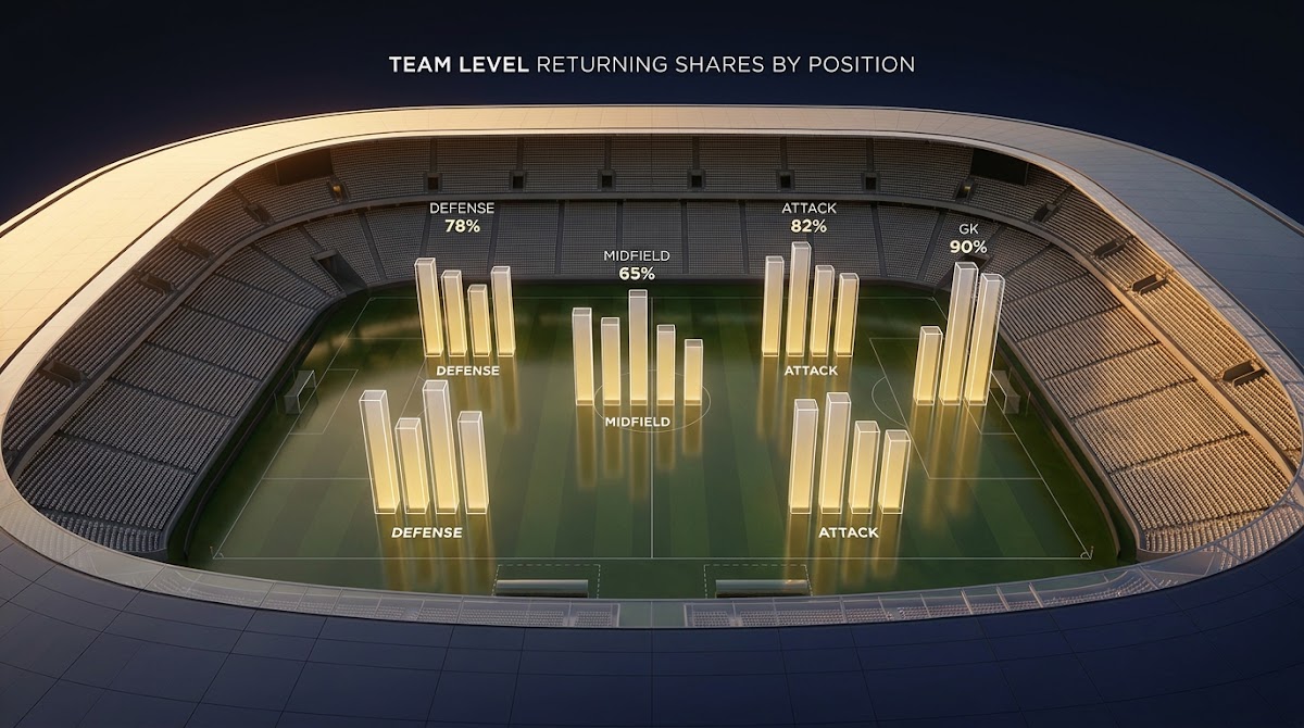
From these inputs the typical ETL process is straightforward: extract prior-year player stats, normalize by team totals to compute each player’s share, map players to current roster status, and then sum shares by position to produce team-level returning shares.

Documenting query versions, recording how you resolve name mismatches, and saving intermediate CSVs are essential reproducibility steps so that analysts can review and update returning-production calculations season to season.

Adjusting returning-production calculations for transfers, redshirts, and graduations

How transfer-portal churn affects raw returning shares

Transfer-portal churn materially changes naive returning shares because contributors from the prior season may exit and incoming transfers can add production that is not visible in last year’s team totals. NCAA trend reporting shows elevated roster churn in recent cycles, so accounting for transfers is a required adjustment rather than an optional refinement NCAA transfer trends report. Alternate real-time tracking endpoints are available from Sportradar transfer tracking.

A practical workflow first flags prior-season contributors who are no longer on the roster by cross-referencing roster announcements, portal declarations and official team lists. Where a confident mapping exists, subtract an outgoing player’s share from the team’s returning total; where uncertainty remains, apply conservative assumptions and document them.

Practical mappings for redshirts and graduated players

Redshirt returns and graduations require clear rules: count returning redshirts as available contributors if they are listed on the active roster and were not exhaustively absent for eligibility reasons, and treat confirmed graduates as non-returning unless the player is explicitly listed as a graduate transfer in the incoming list.

When roster cases remain unresolved, prefer conservative treatment that avoids overstating returning capability; explicitly record those unresolved cases so downstream users understand which teams have higher uncertainty in their returning-production figures.

Translating player-level returns into team-level shares and position weights

Computing team shares from player contributions

Start by aggregating player-level stats into a team total for the chosen metric, compute each returning player’s share as player_stat divided by team_total, and then sum shares for returning players to get the team-level returning share for that metric. Repeat for each metric you track and for each position group.

For example, returning receiving share is the sum of returning receivers’ receiving yards or targets divided by the team’s prior-season receiving yards or targets; the same arithmetic applies to rushing or defensive tackle shares.

Funded Plays Challenges

View FundedPlays Challenges

Position weighting: why QB and receiving production often matter more

Modelers commonly give outsized weight to quarterback and receiving production on offense because those roles concentrate decision-making and volume, while defensive weighting often emphasizes experience and playmaking. This differential treatment is consistent with the way leading preseason frameworks convert returning stats into ratings ESPN SP+ explainer.

To avoid distortions from low-sample contributors, cap extreme individual shares (for example, a single player’s share cannot exceed a reasonable ceiling) and floor tiny shares so that noise from minimal playing time does not swell a team’s computed continuity.

Applying decay weights and multi-year priors in preseason models

Why decay weighting stabilizes signals

Decay weighting places greater emphasis on the most recent season while still leveraging information from older seasons, which increases stability by reducing sensitivity to one anomalous year. This multi-year approach is common in SP+ style models and practical preseason workflows ESPN SP+ explainer.

Simple decay schemes and implementation tips

A straightforward scheme is to use weights such as 0.6 for the most recent season, 0.3 for the prior season, and 0.1 for the season before that, then normalize so the weights sum to one for your returning-production metrics. Choose two or three seasons based on the stability you need and data availability.

When implementing decay, document the chosen weights and test sensitivity by comparing outcomes under alternative weightings; reporting those sensitivity bands helps stakeholders understand how much a single recent season influences the preseason signal.

Validating returning-production signals and avoiding overfitting

Model checks and holdout validation

Robust validation uses holdout seasons to test whether returning-production metrics explain subsequent outcomes after controlling for schedule strength and recruiting. Cross-validation or season-based holdouts let you measure how much incremental variance returning-production features explain versus baseline models.

Evidence linking squad continuity to performance supports including returning-production inputs, but every modeler should check that the feature improves out-of-sample predictions rather than just fitting historical idiosyncrasies Journal of Sports Analytics study on squad continuity.

How squad continuity evidence supports predictive use

Cross-checks commonly include correlation matrices between returning shares and next-season performance metrics, and regressions that control for recruiting class quality; these checks quantify whether continuity carries predictive weight beyond other inputs and thus whether the returning-production signal deserves allocation in your final model.

Practical workflow: example pipeline from raw stats to preseason team ratings

End-to-end steps with checkpoints

An ordered pipeline typically looks like this: pull prior-season player stats from public sources (see Funded Plays homepage Funded Plays), normalize and compute player shares, reconcile each player to current roster lists, adjust shares for confirmed transfers and graduations, apply position weights and decay, and finally integrate the adjusted returning-production features with recruiting and recent performance inputs for a composite preseason rating.

At each step, create checkpoint artifacts such as CSVs of raw pulls, a reconciliation table mapping player IDs to roster status, and unit tests that verify shares sum correctly to team totals; these artifacts make it easier to audit the pipeline and update it as roster information changes; see how Funded Plays evaluations work.

Save reproducible artifacts including a player-shares CSV, a roster-reconciliation sheet, a parameter file with decay weights and position weights, and a short reproducible notebook demonstrating the end-to-end transformation so that others can re-run or adapt your workflow, and see related material on our blog.

Case studies: applying returning production adjustments in two scenarios

Scenario 1: high returning production but QB lost to transfer

Imagine a team that retains a high share of offensive yards and receiving targets but loses its starting quarterback to the transfer portal; the aggregate returning-production number overstates offensive continuity because passing leadership and decision-making have departed. In this case, downgrade quarterback-influenced components and reweight rushing and line continuity while documenting the change and running sensitivity checks to quantify impact NCAA transfer trends report.

Record the altered shares, note assumptions about potential internal replacements or incoming transfers, and run your preseason model under both a conservative no-replacement assumption and a best-case replacement assumption to produce an uncertainty band for the team rating.

Scenario 2: low raw returning production but incoming transfer class bolsters roles

Conversely, a team with low raw returning shares can improve materially if several incoming transfers or returning redshirts occupy major roles. To capture this, add estimated shares for confirmed incoming contributors and document how those estimated contributions were derived, then re-run the weighted aggregation to see how the composite preseason rating moves.

Always keep the estimated incoming contributions separate in your artifacts so that stakeholders can see both a raw returning-production baseline and a transfer-adjusted projection.

Common pitfalls when using returning production and how to avoid them

Top data and conceptual mistakes

Frequent errors include relying on returning-starters flags instead of player-level counts, failing to reconcile transfer-portal moves, double counting snaps for players with multi-role time, and over-weighting an outlier single-season performance without multi-year context.

Mitigations are straightforward: use player-level counting stats, reconcile rosters carefully, cap individual shares to prevent dominance by a single-season outlier, and apply decay to smooth extreme years, following common model practices.

Practical mitigations

Run a short pre-release checklist on every dataset to ensure no double counts, that player shares sum approximately to team totals, that unresolved roster cases are flagged, and that sensitivity to weight choices is reported alongside final ratings.

How returning production complements recruiting and recent performance

Combining signals: recruiting, prior performance, and returning shares

Leading approaches blend returning production with recruiting and recent multi-year performance so that teams with high-rated incoming classes but low returning shares are not penalized unfairly. This blended approach reflects the pragmatic design used in prominent preseason frameworks that balance stability and state-of-program information ESPN returning production rankings.

Practically, give more weight to recruiting when a roster turnover creates clear vacancy at a high-leverage position and lean on returning production when continuity is obvious and role incumbents return.

Communicating returning-production findings: visuals, uncertainty, and transparency

Recommended charts and tables

Useful visuals include stacked bar charts of team returning shares by position, position-weighted change plots that show how applying weights affects team continuity, and uncertainty bands that display results under alternative transfer assumptions and decay weights.

Always publish a short assumptions note describing how transfers, decay weights and roster reconciliation were handled so that readers understand the provenance of the returning-production input and the limits of its interpretation.

Conclusion: practical takeaways for using returning production in preseason analysis

Best practices are simple to summarize: compute returning production from player-level counts, reconcile and adjust for transfers and roster moves, apply decay weights to stabilize signals across seasons, and validate features with holdout tests before integrating into final preseason ratings.

Returning-production inputs are powerful when used responsibly and documented clearly; they provide a transparent, reproducible way to capture continuity that complements recruiting and recent performance while acknowledging the uncertainty introduced by transfers and eligibility changes.