Using Home-Field Advantage in Models: Practical steps and pipelines

What is home advantage and why it matters for prediction models

Definition and typical mechanisms: Using Home-Field Advantage in Models

Using Home-Field Advantage in Models starts with a plain-language idea: teams tend to perform differently when they play at home compared with when they play away. Modelers treat that difference as a location effect that can change expected points, spreads, or win probabilities. Recognizing the effect helps align raw team ratings with observed outcomes and prevents systematic bias when producing forecasts.

Typical mechanisms behind home advantage include crowd influence, travel fatigue, venue familiarity, officiating tendencies, and local environmental factors. Each mechanism can operate at different magnitudes in different sports and on different schedules. Thinking about these drivers helps you choose whether to model a single additive adjustment, a probability multiplier, or a more complex interaction with game-level covariates.

At the modeling level, ignoring venue effects can produce biased baseline probabilities or ill-calibrated spreads, because a neutral baseline does not reflect location-dependent behavior. That bias is especially visible when teams have uneven home and away schedules or when neutral-site games are common. The consequences for downstream calibration and decision-making vary by objective, whether you are optimizing raw probability accuracy, profit-oriented signals, or ranking teams for challenge-style evaluation.

To make the concept tangible, a simple example is useful: if a model predicts a 50 percent chance for a team under neutral assumptions but historical differences show a consistent home uplift, the modeler can encode that uplift either as a points adjustment to spreads or as a direct increase in win probability. The choice between those representations matters for calibration and for how the adjustment interacts with market lines or challenge rules.

How home effects change model baselines

Venue effects shift the baseline for team ratings by adding a location term to the expected outcome. In simple rating systems, you might add or subtract a fixed point value to the home or away team score prediction. In probability models, you might convert that point adjustment to a win-probability delta. Understanding how the baseline moves under different representations is critical for consistent calibration.

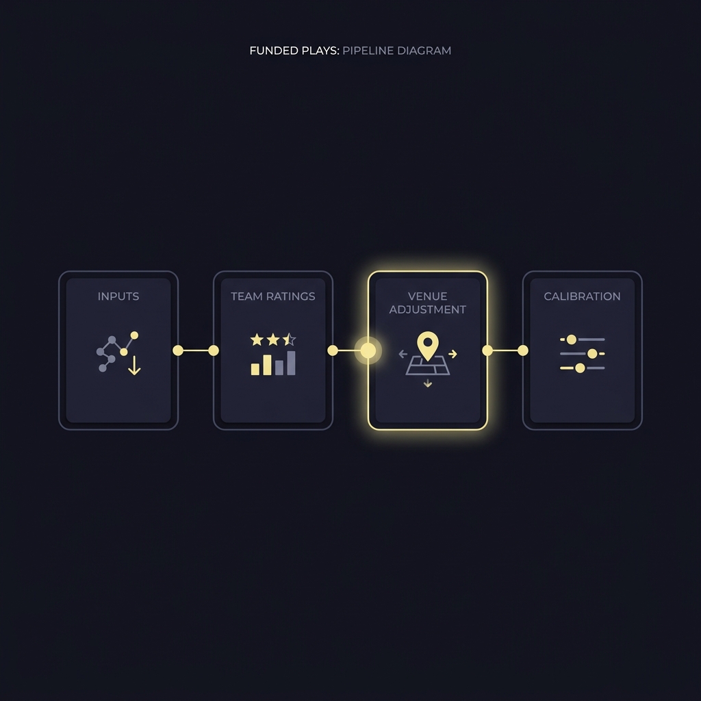
When building a baseline, make the adjustment explicit and record its provenance so you can version and test it later. Avoid implicit adjustments embedded in training data or ad-hoc post-processing that are not tracked; explicit, versioned adjustments are easier to validate and to retire when they stop validating.

Typical empirical indicators that typically reveal venue effects include home/away win splits, scoring differences by venue, patterns in officiating calls, travel distance and rest patterns, and event-level anomalies tied to particular stadiums. These signals are visible at different granularities, from season-level aggregates to play-by-play sequences, and each granularity suggests different modeling approaches. For wider literature coverage, see the systematic review on venue factors in team sports at PMC.

For practical model work, look for consistent patterns across several seasons rather than depending on a single short run. Seasonality, schedule imbalance, and changes in league rules can all move apparent signals from one season to the next. Treat single-season shifts as hypotheses to test rather than stable facts to adopt without validation.

Public and proprietary data sets modelers can use

Useful data types include play-by-play feeds, box scores, full-season schedules with dates and venues, travel itineraries or estimated distances between venues, stadium attributes such as field surface and orientation, and contextual information like weather for outdoor sports. Combining multiple data sources lets you test which mechanisms best explain observed location differences and where to invest modeling effort.

Pay attention to data quality. Play-by-play feeds are rich but can be noisy or inconsistent across providers. Box scores and official schedule data are often cleaner for season-level splits, while proprietary tracking or lineup feeds enable lineup- or possession-level adjustments if you have sufficient coverage. When data are sparse, prefer simpler aggregate adjustments until you can validate higher-resolution models.

How to quantify home advantage: metrics and baseline calculations

Simple metrics: home win rates and points splits

Start with straightforward metrics you can compute from box scores. Compute home and away win rates and average scoring differentials by venue. Convert point differentials to model-friendly adjustments by averaging the difference and mapping it into the units your model uses, such as points for spread models or score margins for expected-value calculations. For discussions of team-level estimation methods see recent work.

When computing raw splits, use clear denominators and report sample sizes. A small number of games at a venue or a short timeframe can produce volatile estimates. Present results with confidence intervals or conservative shrinkage toward a league mean when sample sizes are limited to avoid overreacting to random variation.

Advanced metrics: adjusted plus-minus and lineup-level approaches

For teams and sports with richer play-level data, use adjusted plus-minus or lineup-level models to isolate location from teammate and opponent effects. These approaches estimate location as one of several factors while controlling for which players or lineups are on the field or court. They require larger samples and careful regularization, but they let you detect context-specific venue effects that aggregate metrics mask.

When data permit, compare simple aggregate adjustments with lineup-level estimates to see if the direction and approximate magnitude agree. If they diverge, investigate which matchups or situational contexts drive the difference before adopting a complex adjustment into a production pipeline.

Core framework for integrating venue adjustments into prediction pipelines

Where venue adjustments sit in a multi-stage pipeline

Think of a prediction pipeline as ordered stages: raw inputs, team or player ratings, venue adjustment, and probability calibration. Venue adjustments belong in the stage after you compute your baseline ratings and before final probability calibration. That placement keeps team ratings interpretable and makes it straightforward to test the impact of venue on end metrics without contaminating core ratings.

In practice, implement a modular step or function for venue adjustments so you can switch between additive and multiplicative modes and run controlled experiments. Clear interfaces between stages make it easier to reproduce forecasts, backtest changes, and show results to stakeholders.

Applying additive versus multiplicative adjustments

Decide whether an additive point adjustment or a multiplicative probability adjustment suits your model and your objective. Additive adjustments work naturally in spread models where adjusting predicted points is the intuitive operation. Multiplicative adjustments make sense in probability models that operate directly on odds or likelihoods.

After applying any adjustment, always run a recalibration step on a validation set to preserve calibration. If you add points to the predicted scores, convert the adjusted scores into probabilities and then recalibrate with a calibration curve or isotonic regression to ensure that predicted probabilities remain meaningful and interpretable for downstream decision rules. For practical examples of team-level modeling methods, see team estimation research such as the UEFA-focused study at ScienceDirect.

How adjustment methods differ by sport and market

Examples: soccer, basketball, American football, baseball

Different sports show different patterns because of format, frequency, and substitution rules. Soccer often has lower scoring and limited substitutions, so venue effects may appear more in win-draw-lose splits. Basketball and baseball involve many possessions or plate appearances, so venue effects can be estimated at higher resolution and may be influenced strongly by lineup or starting pitcher choices. American football seasons are shorter with heavier travel impacts, so sample size is a practical constraint early in the season.

Funded Plays Challenges page

See FundedPlays Challenges

Market context also matters. Pre-game markets often incorporate season-level narratives that are stable over time, while in-play models require micro-level modifiers that react to game state and fatigue. Choose the temporal resolution of your venue adjustment to match the market you intend to serve or to evaluate against.

Market differences: pre-game lines vs live models

For pre-game models, season-level or opponent-adjusted home splits are often sufficient and easier to validate on holdouts. Live models usually benefit from possession-, lineup-, or minute-level modifiers that reflect fatigue, substitution patterns, and evolving matchups. The operational cost and data requirements of live adjustments are higher, so balance expected gain against complexity and latency.

Game-level factors to model alongside home advantage

Travel, rest, altitude and climate

Game-level modifiers interact with venue effects. Travel distance and rest days can amplify or reduce a location uplift, especially on tightly packed schedules. Altitude and local climate can be material in some contexts and virtually irrelevant in others; include them when you have plausible mechanisms and supportive data.

When adding these covariates, code them consistently and avoid overfitting. For example, compute travel distance with a reproducible method and treat unusual travel patterns as flags to be investigated rather than immediate drivers to tune in production models.

Roster changes and lineup continuity

Roster availability alters how a venue effect plays out. Late scratches, injury reports, and sudden lineup changes can materially shift expected outcomes in the short term. Include simple binary indicators or more detailed lineup-quality covariates when those signals are available and reliable.

For many use cases, a compact set of game-level modifiers yields most of the practical benefit: travel distance, rest differential, key-player availability, and whether the game is at a neutral site. Use those as a first layer and expand granularity only if validation shows consistent improvement.

Validating home adjustments: backtesting and cross-validation strategies

Designing proper holdouts that respect schedule structure

Design validation so it respects temporal and schedule structure. Use season holdouts, time-aware cross-validation folds, or block validation that prevents leakage from later to earlier games. Avoid random shuffles that mix training and test games across time because schedule-dependent signals can then leak and give overly optimistic estimates of improvement.

Record the exact holdout plan and enforce it in automated pipelines so future re-runs use the same splits. Reproducible validation guards against accidental overfitting and makes it easier to compare model versions objectively. See example discussions and posts on the Funded Plays blog for pipeline writeups.

Measure calibration with Brier score and with calibration plots, and track log loss or cross-entropy for probability models. For decision-focused models, include profit-style KPIs that match your real objective. Report both statistical improvement and practical effect size so that small, statistically significant changes do not get mistaken for useful operational gains. See a related evaluation example at how evaluations work.

Complement metric tracking with simple visual checks such as predicted versus observed splits by venue and season. When a change changes calibration patterns more than it improves discrimination, prefer recalibration techniques rather than wholesale model changes.

A decision checklist: when to apply, adjust, or ignore home effects

Quick decision flow for modelers

Use a short decision flow: confirm adequate sample size, test season consistency, run a baseline experiment, and accept only when validation metrics justify deployment. Keep the flow simple and document each decision to maintain traceability and to revisit choices when conditions change.

Document thresholds for action. For example, require consistent improvement on holdout calibration and a minimal practical effect on your business metric before making the adjustment live. If the improvement is ambiguous, prefer a conservative, versioned rollout with close monitoring.

Common thresholds and red flags

Red flags include sparse data, inconsistent season-to-season signals, and situations where other covariates explain the apparent venue effect. If you see a large venue uplift but also notice that a team faced much weaker opponents at home, investigate confounding before accepting the uplift as a true location effect.

When in doubt, prefer shrinkage toward a league or sport mean and require repeated validation across seasons before relying heavily on a venue adjustment in high-stakes decision systems.

Common mistakes and pitfalls when modeling home advantage

Overfitting to recent streaks

One common mistake is overfitting to short-term streaks or a few unusual games. Short horizons produce noisy estimates; use regularization, shrinkage, or Bayesian priors to stabilize estimates and to express uncertainty about small-sample signals.

Another operational issue is failing to monitor for rule changes or schedule shifts that change the baseline. These structural changes require revisiting assumptions before continuing to rely on historical adjustments as if something fundamental did not change.

Confounding venue with opponent strength

Teams that play easier opponents at home can create spurious home effects in raw splits. Control for opponent strength and schedule imbalance when possible. Regression with opponent controls or matched-pair comparisons are two practical ways to reduce this confounding risk.

Operationally, also avoid misusing raw win rates without inspecting matchup patterns. Where confounding is suspected, run sensitivity checks that hold opponent quality constant and look for persistence in the location signal.

Practical walkthrough: applying venue adjustments in an NFL model

Step-by-step data and calculation plan

For an NFL model, collect these minimal inputs: full season schedules with venues and dates, team ratings or baseline spreads, rest-day information, approximate travel distances, and accessible injury or availability notes. Start with season-level home/away splits to create an initial additive points adjustment and document sample sizes for each estimate.

Compute a baseline additive adjustment by averaging observed point differentials by venue after controlling for opponent strength with a simple regression or matched comparison. Use shrinkage when sample sizes for particular teams or venues are small. Record the adjustment as a versioned parameter that you can toggle for experiments.

Run holdout experiments where you compare the forecasted spread and the adjusted spread across the same validation set, then convert adjusted spreads into probabilities and check calibration. Track Brier score, calibration curves, and any profit-like metrics relevant to your objectives. Prefer results that are robust across multiple seasons rather than a single test set before deployment.

Handle neutral-site games explicitly by tagging them and modeling them as neither home nor away or by estimating a separate neutral-site parameter if data permit. For early-season weeks where samples are small, downweight venue adjustments and require stronger evidence before applying aggressive corrections to forecasts.

Practical walkthrough: differences for NBA and baseball models

Why home effects manifest differently in high-frequency sports

In sports with dense schedules such as the NBA and MLB, teams play many games in short periods, and travel patterns can create predictable fatigue cycles. High-frequency data allow you to estimate short-term modifiers such as rest differentials and minute-load effects, but they also raise the risk of overfitting to transient patterns. Balance granularity with conservative regularization.

Because data are abundant, consider estimating location effects at multiple levels: team-season, lineup, or player-season. Compare results across levels to determine where marginal gains justify added complexity and computational cost.

Specific tactics for lineup and pitcher effects

In the NBA, lineup rotation and matchup minutiae make lineup-level effect estimation valuable. Use lineup usage data and plus-minus style models to detect how certain lineups perform in different arenas. Regularize estimates heavily and aggregate to lineup clusters when individual lineup samples are small.

In baseball, starting pitcher identity is often the dominant short-term driver. Model home effects conditional on the starting pitcher when you have sufficient depth, or include pitcher-specific interactions with venue when pitcher data are essential to forecasts. For teams with substantial pitcher turnover, consider a hierarchical approach that pools information across pitchers and teams.

Implementation checklist and quick experiments to run

Minimum viable tests to validate adjustments

Start with a minimum viable experiment: compute season-level home/away splits, estimate a simple additive adjustment, apply it to a validation holdout, and measure calibration and your main business KPI. Keep changes small and track them in version control so you can roll back if validation does not support the change.

Ensure you log experiment metadata: dates, folds, sample sizes, and configuration parameters. That logging helps avoid confirmation bias and makes it easier to reproduce and audit results later. Store experiment artifacts on your site or repository such as Funded Plays.

Short experiments for model improvement

Run three short experiments: (1) a season-level additive adjustment applied uniformly, (2) a travel-distance interaction that changes the adjustment by rest differential, and (3) a lineup- or pitcher-level modifier that activates only when sample thresholds are met. Compare their performance on the same holdout and prefer the simplest approach that produces consistent improvement.

When running experiments, maintain a conservative rollout policy. Favor staged deployment and close monitoring rather than full immediate replacement of baseline models when the new method yields modest gains.

Monitoring, recalibration and keeping venue effects up to date

Triggers that suggest recalibration

Recalibrate when you detect drift in calibration metrics, when league rules or schedules change, after substantial roster turnover, or when officiating patterns shift. Automated alerts on calibration degradation and sudden shifts in venue-specific residuals help catch issues early.

Keep a cadence for scheduled re-evaluation, for example at season boundaries or after major rule changes. Combine scheduled reviews with event-driven checks so you neither overreact to noise nor miss meaningful changes.

How to version and monitor adjustments

Use version control for adjustment parameters and keep experiment metadata with each version. Monitor both statistical metrics and practical KPIs, and maintain dashboards that show venue-specific residuals and calibration plots. When an adjustment stops validating, consider downweighting it or retiring the parameter rather than leaving it active by default.

Document rollback criteria and ensure your pipeline supports quick reversion to previous versions when necessary. Operational readiness and clear guardrails reduce risk when venue effects interact with other rapidly changing model components.

Conclusions and next steps for modelers

Key takeaways

Home adjustments matter because venue can shift expected outcomes and because untested adjustments can both improve and harm model performance. Measure cautiously, validate rigorously, and prefer explicit, versioned adjustments that you can audit and retire. Align your approach with the sport and the market you serve.

Where to focus efforts next

Prioritize data collection and a small set of minimum experiments: a season-level additive test, a travel interaction, and a player- or lineup-aware probe when data volume permits. Require consistent, out-of-sample improvement before adopting any adjustment in production.

Keep a disciplined validation plan, log experiments, and maintain conservative rollouts. That approach preserves model interpretability and reduces operational risk while allowing measured gains from modelling venue effects.