Using Confidence Ranges Instead of Exact Predictions: Practical Guide for Sports Forecasts

What confidence ranges are and why they matter, Using Confidence Ranges Instead of Exact Predictions

Many sports forecasts start as single numbers: a win probability, a predicted score, or a projected point total. Using Confidence Ranges Instead of Exact Predictions encourages reporting an interval or a set of percentiles around that number so readers understand the uncertainty around the outcome. That shift helps decision makers treat the forecast as information about risk rather than as a guaranteed outcome.

In plain terms, a confidence interval describes uncertainty about an estimated parameter, while a prediction interval covers where a future observation is likely to fall. Percentile ranges, such as the 10/50/90 trio, give a compact way to report the distribution of possible outcomes so users can see a plausible low, median, and high case; these three percentiles are commonly used in applied forecasting work and complement standard interval definitions described in statistical references NIST statistical intervals guide.

Point estimates can be misleading because they hide variability and encourage overconfidence. When a model reports only its single best guess, users may act as if that outcome is certain, leading to riskier staking, suboptimal lineup choices, or poor contest-entry decisions.

One short example: for a matchup forecast, publishing a 10/50/90 probability for the favorite to win (say 30/55/80 percent) gives a clear sense of how likely different outcomes are. A bettor or contest entrant can then use the percentile spread to size stakes or choose entries while acknowledging that the median is just one summary of a broader distribution.

Why probabilistic ranges are best practice today

By 2026, best practice in forecast communication recommends probabilistic ranges as the default because ranges convey uncertainty needed for informed decisions and reduce misinterpretation common with single-point estimates. Verification guidance from operational forecasting organizations emphasizes ranges and probabilistic approaches as the preferred way to present forecasts to users who must manage risk ECMWF forecast verification.

Ranges support calibrated decision thresholds: instead of treating a 60 percent point estimate as a yes-or-no signal, a team can define actions that depend on percentile bands, such as entering a contest only when the 10/50/90 spread is narrower than a threshold or when the lower percentile exceeds a risk limit. This lets forecasters set rules that map uncertainty to operational choices rather than relying on a single, sometimes misleading point.

It is important to add a caution: publishing ranges does not guarantee outcomes. Ranges must be paired with evaluation, out-of-sample checks, and routine monitoring to ensure that the stated percentiles reflect real-world performance over time.

The twin pillars: calibration and sharpness explained

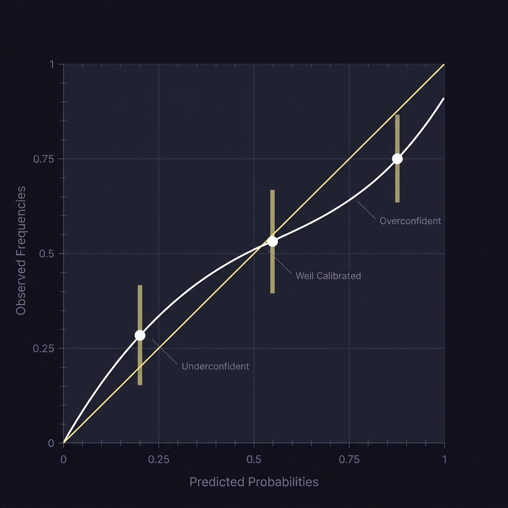
Two key properties determine whether probabilistic ranges are useful: calibration and sharpness. Calibration, often called reliability, asks whether stated probabilities match observed frequencies. For example, if many events were assigned a 70 percent chance, about 70 percent of them should occur for the model to be well calibrated. Verification pages and practical guides stress checking calibration first when assessing forecast quality NWS verification.

Sharpness refers to the concentration of the predictive distribution. All else equal, narrower ranges are preferred because they give more informative guidance, but only when calibration holds. A very sharp range that systematically misses observations is worse than a wider, reliable range. The goal is to balance sharpness and calibration so that ranges are both informative and trustworthy.

Reliability diagrams and calibration curves are practical visual tools to spot miscalibration. These plots compare predicted probability bins to observed frequencies; deviations indicate overconfidence or underconfidence. When a reliability curve veers away from the diagonal, forecasters should consider recalibration or revising model assumptions rather than using narrow ranges that mislead users.

How to construct confidence and prediction ranges

Classical statistical intervals and quantile regression

Classical methods provide a baseline: confidence intervals quantify uncertainty about estimated parameters and prediction intervals incorporate future observation variability. For many models, simple analytic formulas exist for prediction intervals; these remain a sound starting point and are described in standard references on intervals and forecasting Forecasting: Principles and Practice.

Quantile regression is a practical, model-agnostic way to estimate percentiles directly. By predicting a chosen quantile, you can construct 10/50/90 percentiles from separate quantile models or from a model that supports multiple quantiles. Quantile approaches work well when residuals are heteroskedastic or distributions are skewed, common situations in sports outcomes.

Conformal prediction for distribution-free intervals

Conformal prediction creates prediction intervals with finite-sample coverage guarantees under exchangeability, meaning intervals are valid without assuming a specific distribution for residuals. This property makes conformal methods appealing for sports datasets where distributional assumptions often fail. For a practical introduction and intuition on conformal methods, recent tutorials summarize how to apply them in applied settings conformal prediction survey, classic tutorials include Shafer's tutorial and an ACM tutorial.

Conformal methods are easy to combine with modern machine-learning models: after fitting a point or quantile model, a conformal wrapper adjusts intervals so they meet nominal coverage on held-out data. The trade-offs are familiar: conformal intervals tend to be robust but may be slightly wider than parametric intervals if those parametric assumptions hold exactly. See a practical walkthrough nixtlaverse conformal tutorial.

Evaluating ranges: scoring rules, coverage, and out-of-sample checks

Proper scoring rules let you measure both calibration and sharpness in one number. The Brier score and log loss are standard choices: the Brier score handles bounded outcomes like win probabilities, while log loss is sensitive to confidence in probabilistic predictions. Verification resources recommend using these scores to track model performance and compare alternatives ECMWF forecast verification.

Coverage tests compare the nominal percentile level to empirical frequencies. If you report a 90 percent interval, approximately 90 percent of observations should fall inside that interval when checked out-of-sample. Compute empirical coverage on a held-out season or using time-respecting cross-validation, and treat large, systematic gaps as signs that recalibration or alternative interval methods are needed.

Reliability diagrams work hand in hand with scores: a good score with a flat but biased reliability curve suggests recalibration is needed, while a degraded score accompanied by widening intervals could indicate model drift. Routine out-of-sample checks are essential for sports contexts where seasonality and roster changes can shift underlying distributions.

Tools, pipelines, and visualizations that make ranges practical

Practical toolkits now include probability calibration utilities and reliability plotting functions that make it straightforward to compare raw and calibrated outputs. For example, calibration modules in popular ML libraries provide utilities to fit calibration transforms and plot reliability curves for easy inspection scikit-learn calibration docs.

To operationalize ranges, set up a simple pipeline: generate out-of-sample predictions, compute quantiles or prediction intervals, measure empirical coverage and scores, and store results for trend monitoring. Automate alerts when empirical coverage drifts from nominal levels or when proper scores degrade materially so you can investigate model or data issues before decisions rely on stale ranges.

Funded Plays Challenges page

Get the checklist

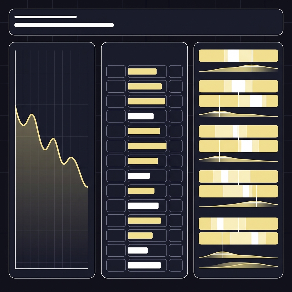
Dashboards that combine reliability diagrams, time series of Brier scores, and coverage tables make it easy for analysts and decision makers to see where models remain reliable and where retraining or recalibration is necessary. For sports forecasts, include team- or player-level breakdowns to detect localized problems hidden by aggregate metrics.

Translating ranges into decisions for sports forecasts

Percentiles like 10/50/90 translate naturally into action rules. For entry or staking decisions, you might require that the lower percentile exceed a minimum confidence threshold before increasing exposure, or scale stake size by the interpercentile range so narrower spreads justify larger stakes. The verification guidance recommends validating these rules with out-of-sample tests before relying on them operationally NWS verification.

Always check empirical coverage first: if the 10 percentile is supposed to be a 10 percent tail but empirically contains 20 percent of outcomes, your threshold will understate risk. Combine ranges with disciplined bankroll management so decision rules respect drawdown limits and do not assume ranges are perfect forecasts.

Common mistakes and how to avoid them

Forecasters often report narrow intervals that look good in-sample but fail out-of-sample because of overfitting or ignored non-stationarity. A quick sanity check is to compute empirical coverage on unseen data and compare it to nominal levels; consistent misses suggest recalibration or a different interval method.

Another frequent error is confusing confidence intervals for parameters with prediction intervals for future outcomes. Use prediction intervals or percentile forecasts when the objective is to describe possible game-level outcomes, and reserve confidence intervals for statements about model parameters or long-run averages.

Dataset issues are common in sports: small samples, roster changes, and non-stationary effects can all undermine coverage. Regular monitoring, conservative interval widths when data are sparse, and retraining schedules keyed to regime changes help avoid fragile ranges that mislead decision makers.

Concrete sports forecasting scenarios and short walkthroughs

Scenario A, match-level percentiles: compute predicted distributions for each game using a suitable model or quantile regressions, then extract the 10/50/90 percentiles. On a held-out validation set, count how often the actual result falls below the 10 percentile and above the 90 percentile to compute empirical coverage. If coverage aligns with nominal levels, you can use the percentiles to define entry thresholds; if not, recalibrate first. This step-by-step practice mirrors verification workflows used in operational forecasts ECMWF forecast verification.

Scenario B, season monitoring and recalibration: log proper scores and coverage each week across the season. If the Brier score trends worse and coverage slips, isolate whether data drift, model stale features, or structural breaks like injuries are the cause. Apply a recalibration transform or re-estimate quantiles on a rolling window and re-check coverage before redeploying forecasts.

Both scenarios illustrate responsible practice: ranges inform decisions only when their empirical properties are verified. In challenge environments where users demonstrate forecasting skill, these checks help maintain a level playing field and prevent overconfident entries based on untested ranges.

Conclusion: a short checklist for moving from points to ranges

Quick checklist: pick an interval method, calibrate probabilities, test out-of-sample coverage, monitor proper scores such as Brier and log loss, and iterate when drift appears. These steps help ensure ranges remain informative and reliable for operational decision making.

Remember that ranges improve clarity and reduce overconfidence but do not guarantee outcomes. Continued verification and conservative risk management are essential parts of using probabilistic forecasts in sports.