Travel Distance as a Sports Analytics Variable — A Practical Guide

What travel distance means in sports analytics: Travel Distance as a Sports Analytics Variable

Definitions: distance, travel burden, and related terms

Travel distance, in the context of sports analytics, refers to a measurable quantity that captures how far a team or player travels between venues for competition. The phrase Travel Distance as a Sports Analytics Variable signals treating that measured quantity as an input to models rather than as a descriptive label.

Related terms clarify different aspects of travel. Time zones describe longitudinal shifts that can cause circadian disruption. Travel duration captures the elapsed door-to-door time, and travel burden combines distance, duration, and contextual friction such as layovers or overnight travel. Distinguishing these terms helps an analyst decide which element to capture for a specific question.

Why travel is considered a variable rather than a simple fact

Analysts treat travel as a variable because its measured value can vary across games, players, and seasons and because it may interact with other model inputs. As an input feature, travel distance can function as a numeric covariate, a binary flag, or a moderator that changes the relationship between other predictors and the outcome.

Common uses of travel-derived variables include team-level effects, where aggregated travel load is aligned to a team-game record, player-level effects that account for individual minutes and time on the road, and scheduling analyses that look at clusters of travel across a season. Clear definitions at the outset reduce confusion when aligning travel measurements with performance windows.

Funded Plays Challenges

View Challenges

Why analysts care about travel distance

Potential mechanisms: fatigue, circadian disruption, logistics

Travel is plausibly linked to performance through several mechanisms, including physical fatigue from transit, circadian disruption from time zone changes, and logistical friction such as late arrivals and disrupted practice routines. Treat these mechanisms as hypotheses to test rather than established causal facts.

When considering mechanisms, use domain knowledge to identify plausible mediators like sleep quality, meal timing, and practice time. Analysts can then seek proxy variables or operational data to represent those mediators rather than relying solely on distance as a surrogate.

When travel matters more: short turnarounds, long-haul trips, international fixtures

Not all travel is equally relevant. Short turnarounds between games amplify the effect of incremental travel burden because recovery time is limited. Long-haul trips that cross multiple time zones are more likely to introduce circadian misalignment. International fixtures add customs, visa logistics, and variable accommodation quality that can increase burden.

Context matters by sport, schedule format, and team resources. For example, frequent regional travel in a dense schedule differs from occasional long-haul travel that requires targeted recovery interventions. Phrase conclusions carefully and test them against the data available for the specific sport and calendar.

How to measure travel distance: data sources and metrics

Distance metrics: great-circle, driving distance, travel time

Common distance metrics include great-circle distance, which estimates the straight-line distance between two coordinates; route-based driving distance, which follows road or rail networks; and estimated travel time, which can incorporate typical traffic or flight durations. Each metric captures a different notion of effort and realism.

Great-circle distance is easy to compute and reproducible, but it ignores routing constraints and airport locations. Route-based distance is more realistic for ground travel but requires routing data. Estimated travel time begins to capture the actual burden on players but depends on assumptions about transit mode and schedules.

Data sources: stadium coordinates, routing APIs, official schedules

Reliable inputs start with accurate venue coordinates and official game schedules. Geocoding public stadium names to latitude and longitude is a standard first step. For route distances or travel times, routing APIs provide programmatic routes; historical flight schedules or public transit data help estimate typical durations.

Trade-offs include ease of computation, cost, and reproducibility. If reproducibility is a priority, prefer static geocoded coordinates and document the geocoding provider and timestamp. If realism is more important, route-based measures or scheduled flight durations may better capture travel time at the expense of API costs and extra complexity.

Modeling approaches: from simple covariates to engineered features

Simple covariates: numeric distance, binary travel indicator

Start with simple inputs. A numeric distance variable or a binary away-travel indicator can be informative baseline covariates. These inputs are straightforward to compute and interpret, and they serve as useful comparison points when testing more complex features.

Simple covariates reduce the risk of overfitting in small samples and help clarify whether travel has a detectable marginal association with outcomes before adding engineered features.

Engineered features: cumulative travel load, nights away, time-zone shifts

Engineered features capture richer patterns. Examples include a rolling cumulative travel load that sums distance over recent games, a nights-away counter to capture disrupted sleep, and time-zone shift counts to model circadian displacement. Interaction terms between travel features and rest days can reveal conditional effects.

When adding engineered features, monitor multicollinearity and consider regularization. Many travel-derived variables will be correlated with one another and with calendar variables, so use penalized models or variable selection to avoid unstable estimates.

Integrating travel distance into team- and player-level models

Different unit of analysis: team-game vs player-game

Unit alignment matters. Team-game models aggregate travel variables to the team level and align them with team performance metrics. Player-game models require assigning travel exposure at the individual level, accounting for games missed, partial rotations, and late arrival of single players.

When translating team travel to player exposure, decide whether to assign the team travel value to every active player for that game or to weight it by minutes played or roster presence during the trip. The choice depends on the question and the data available.

Hierarchical approaches and random effects

Hierarchical models allow pooling across teams or players while permitting individual differences in travel sensitivity. Random effects can capture baseline team or player tendencies, while travel coefficients can be allowed to vary by group to reflect heterogeneous responses.

Practically, a multi-level model might include team-level random intercepts and player-level random slopes for travel exposure. These structures help stabilize estimates when some teams or players have sparse travel patterns.

Decision criteria: when to include travel distance in an analysis

Signal-to-noise and sample size considerations

Evaluate whether the expected signal-to-noise ratio justifies the complexity of adding travel variables. If sample sizes are small or travel patterns are clustered, travel effects may be hard to estimate precisely. Use power thinking and consider pre-registering an ablation test to quantify incremental value.

Checklist items include hypothesized mechanism, expected direction of effect, variability in travel exposure across observations, and available sample size to detect plausible effect magnitudes.

Cost-benefit: complexity vs marginal predictive gain

Run a quick ablation test: compare a baseline model to a model that adds a small set of travel features and measure the change in out-of-sample performance. Small predictive gains may not justify the cost of collecting and maintaining detailed travel data.

Document assumptions and run sensitivity analyses. If travel features are highly correlated with other predictors, the marginal gain may be negligible even if travel has conceptual relevance.

Practical steps: preparing travel data for modeling

Data pipeline: ingestion, cleaning, enrichment

Construct a simple pipeline: ingest official schedules, geocode venue names to coordinates, compute pairwise distances or travel times, and join those features to your game or player records. Automate data pulls and version outputs to ensure reproducibility.

Enrichment steps can include adding time-zone offsets, typical flight durations between major airports, and local transit times from airport to venue where relevant. Each enrichment increases realism but also the maintenance burden.

Perform basic quality checks: verify coordinates against official venue pages, inspect extreme values for mis-geocoded locations, and check for double-headers or neutral-site games that require special handling. For reproducibility, store raw inputs and processed outputs with timestamps and notes about data providers.

Record assumptions such as whether driving or flying is the assumed mode between particular city pairs and include that decision in metadata accompanying the feature table.

Common pitfalls and confounders to watch for

Mistaking correlation for causation

One common error is using distance as a proxy for fatigue without measuring intermediate variables like sleep or recovery. Distance may correlate with other factors such as opponent strength or travel resources that actually drive observed effects.

Diagnose causal uncertainty with stratified analyses and placebo tests. For example, examine whether distance predicts outcomes in contexts where travel burden should logically be irrelevant to identify spurious correlations.

Collinear features and omitted variable bias

Travel variables can be collinear with schedule density, rest days, and opponent strength. Omitted variable bias can distort estimated travel effects if important confounders are not included. Regularized models, stratification, and sensitivity checks are practical means to assess robustness.

Keep clear documentation of potential confounders and run robustness checks that add or remove correlated predictors. When plausible confounders are unavailable, interpret travel-related coefficients with caution.

Example scenarios and short case studies

Scenario A: short rest, regional travel in basketball

Imagine a team that plays three games in five days, with two regional trips by bus. Relevant features include days since last game, driving distance, number of nights away, and minutes played by key starters. A sensible approach is to start with a numeric distance measure, add a short-rest indicator, and test interactions between rest and distance.

Quick checks include comparing the effect estimate for this team against a pooled estimate and running a placebo test on games with similar rest patterns but no travel to see if the travel variable captures unique variance.

Scenario B: long-haul international flight in soccer

For an occasional long-haul match that crosses multiple time zones, candidate features include time-zone shifts, scheduled flight duration, and arrival time relative to kick-off. Because these events are rare, a hierarchical model that borrows strength from other teams or seasons helps estimate effects without overfitting to a handful of cases.

Operational checks include confirming whether the team chartered a flight or used commercial travel and whether they scheduled an extra training day. Those operational choices can materially change the expected burden associated with a long flight.

Interpreting results: effect sizes, uncertainty, and communication

Translating model coefficients into practical meaning

Translate travel coefficients into operational terms the audience understands, for example by expressing the estimated change in outcome probability or expected points per unit of distance. Avoid presenting such translations as definitive causal effects without supportive auxiliary data.

When converting coefficients, present clear caveats about assumptions and the reference levels used for comparisons. Use conservative language that acknowledges uncertainty in measurement and omitted variables.

Reporting uncertainty and limits

Report confidence intervals or credible intervals and discuss limits of inference. Make it explicit whether estimates reflect within-team variation, between-team differences, or a pooled average that mixes both sources of variation.

Recommend that coaching staff and operations treat model outputs as one input among many and that any operational changes be piloted and evaluated prospectively when possible.

Operational considerations: scheduling, rest, and logistics

How operational choices mediate travel effects

Operational levers such as charter flights, staggered travel, pre-game rest protocols, and choice of hotels can mediate the relationship between travel and performance. Analysts should document whether teams used charters or commercial flights and any organized rest strategies around travel.

Where possible, include these operational indicators in models as additional covariates or interaction terms. These variables often offer stronger explanatory power than raw distance alone.

Collaborating with operations staff for better data

Ask operations staff for non-sensitive aggregated data such as flight departure and arrival times, layover counts, and number of hotel nights. Frame requests around how the information improves model validation rather than as a remote monitoring effort.

Be mindful of privacy and data governance. When working with granular player movement data, agree on anonymization, retention limits, and access controls before integrating such data into analytical pipelines.

How to put it into practice: recommended workflow and checklist

Minimal viable travel model

Minimal steps: obtain the official schedule, geocode venues, compute straight-line distance for each away game, add a binary away flag, and run an ablation comparing baseline and travel-augmented models. Keep the initial feature set small so you can clearly assess marginal value.

Document the baseline model structure and the exact columns added for the travel test. If the ablation shows consistent improvement out of sample, iterate toward richer features.

Advanced pipeline checklist

Advanced steps: route-based distances or estimated travel times, time-zone shifts, rolling cumulative travel load, nights away, and interaction terms with rest days. Use hierarchical models if individual-level or rare-event heterogeneity is expected. Run robustness checks and place results in a version-controlled report.

Always store raw inputs, intermediate tables, and final features with version metadata. This practice makes it possible to reproduce results and to revisit assumptions as new operational data becomes available.

Summary and next steps

When travel distance is worth the effort

Travel distance is worth including when there is a credible mechanism, sufficient variability in exposure, and enough samples to detect plausible effects. If those conditions are absent, a minimal model with a simple travel flag is an appropriate first step.

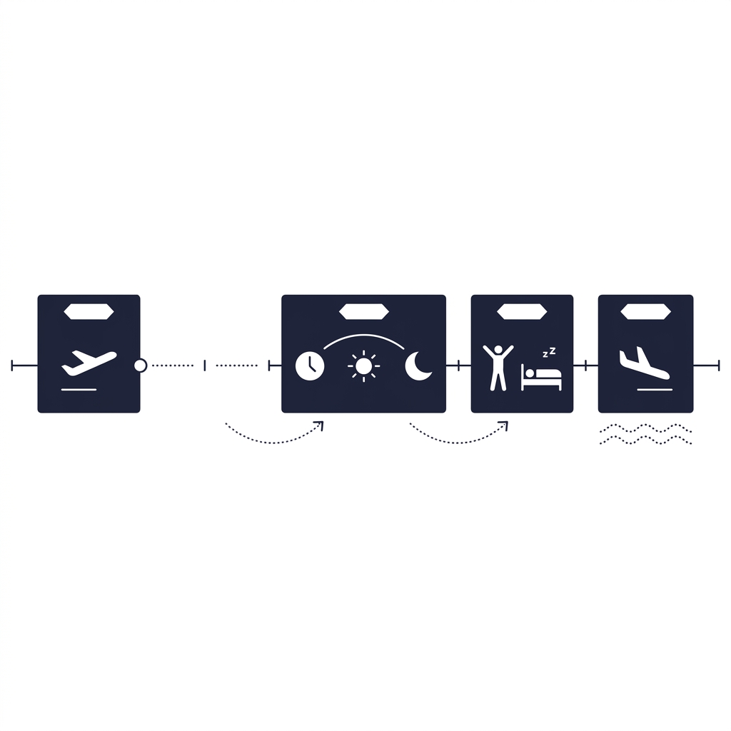
Next steps: run a small ablation test, collect a shortlist of operational variables to enrich the model, and document sensitivity checks. Prioritize reproducibility and conservative interpretation when communicating results.

To test effects in your data, start with a pre-specified analysis plan, run holdout validation for predictive checks, and use stratified or placebo analyses to probe causal assumptions. Iteratively expand the feature set only when initial checks suggest added value.

Continued collaboration between analysts and operations teams improves both feature quality and the interpretability of results. Treat travel-derived variables as hypotheses to explore, not as final answers.