

How to Track Whether Your Model Has a Real Edge: overview and why it matters
When teams ask, "How to Track Whether Your Model Has a Real Edge" they mean something specific: persistent, deployment-relevant predictive value that translates into repeatable decisions rather than a one-off in-sample win. Start by treating an edge as a statement about stability over time and relevance to the business decision you need the model to support, rather than a single high score during development.
Many early claims of an edge collapse when the model meets live data because the original evaluation ignored temporal structure, selected among many candidate models, or failed to separate tuning from holdout testing. Time-aware evaluation avoids these pitfalls by preserving the order of events and testing approaches that mimic how the model will be used.
Practice time-aware validation in a structured challenge environment
Apply the same time-aware, repeatable checks you will use in production before you call a result an edge. Treat validation as a control process, not a one-off report.
To map validation to decisions, distinguish predictive accuracy measures from economic or operational value: a good classification metric does not always imply positive business outcomes, and a small, stable improvement in a target metric can be more valuable than a large but unstable gain.
Practically, you can frame evaluation around deployment objectives, choose metrics that reflect those objectives, and design tests that respect how data arrives in time. For time-aware tooling and the mechanics of rolling evaluation, resources on time-series cross-validation offer concrete guidance for building folds that mimic deployment timing time series cross-validation
Key definitions and context: training, validation, and truly out-of-sample periods
Clear temporal separation is the foundation for credible claims about an edge. The training set is where you fit model parameters and tune routine settings. A validation set supports hyperparameter choices and early stopping. A truly out-of-sample holdout is reserved until final evaluation and should never influence model tuning.
Non-stationarity means the data-generating process changes over time, and that can make a model that looked good in one era fail in the next. Rolling windows and time-aware folds help by repeatedly testing the model on forward slices that reflect how performance evolves with fresh data, which reduces look-ahead bias and produces more realistic estimates of durability cross-validation guidance
How to Track Whether Your Model Has a Real Edge: walk-forward and time-series cross-validation explained
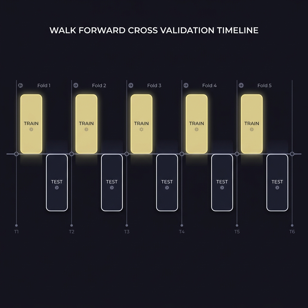
Walk-forward validation, also known as rolling-origin evaluation, advances training and test windows through time so each fold approximates a deployment interval. In practice you train on an initial window, test on the immediately following period, then expand or slide the window and repeat the cycle. This pattern creates sequential out-of-sample tests that reveal stability and sensitivity to temporal changes. For a practical tutorial on using walk-forward methods, see Machine Learning Mastery.
One common reader question is how large each fold should be and how often to update the model to balance stability against responsiveness. A practical guide on Medium explores walk-forward validation and implementation considerations for varying fold sizes Understanding Walk Forward Validation.
Use time-aware validation such as walk-forward folds, choose metrics tied to business outcomes, quantify uncertainty with bootstrap and permutation tests, correct for selection bias, and maintain post-deployment monitoring to detect drift and decay.
Decision choices for window size and update cadence should reflect the pace of change in your problem and your deployment constraints. If outcomes shift slowly, larger windows with less frequent updates reduce variance in estimates. If the environment is fast-moving, use shorter windows and more frequent retraining. Time-series cross-validation methods describe these trade-offs and show why random k-fold splits are inappropriate for ordered data because they mix future information into training sets time series cross-validation
Walk-forward mechanics are straightforward to implement: define your origin, choose a training and testing span, then iterate the train-test pair forward. Record performance per fold and examine stability across folds to identify where performance breaks down or where retraining cadence matters. Those per-fold summaries are more informative than a single aggregated metric when you want to judge durability.
Designing robust backtests that mirror deployment
Robust backtests separate data into stages and avoid contaminating later evaluations with information that would not be available at prediction time. A practical pattern is staged evaluation: use a development window for model building, a validation window for tuning, and a final holdout that remains untouched until you have a finalized pipeline. This staged approach reduces the risk of overly optimistic results caused by in-sample selection.
Rolling windows and simulated live runs help you see how a model behaves when it is reissued repeatedly on new data. Simulated live execution means you run the model as if you were deploying it: generate predictions on the next period using only past data, record outcomes, then update the model according to your chosen schedule. That simulation reveals operational issues and performance decay that stationary backtests miss time series cross-validation
Practical checks to detect look-ahead bias include verifying feature construction is forward-looking, ensuring timestamp alignment for labels and covariates, and logging every data transformation with the exact source and code version. These simple audits often catch pipeline leaks that otherwise invalidate a backtest.
Practical checks to detect look-ahead bias include verifying feature construction is forward-looking, ensuring timestamp alignment for labels and covariates, and logging every data transformation with the exact source and code version. These simple audits often catch pipeline leaks that otherwise invalidate a backtest.
Choosing the right metrics for your goal
Metric selection must follow the decision you expect the model to support. For classification probabilities, choices like ROC-AUC, log loss, and the Brier score capture different aspects of predictive quality: discrimination, calibrated probabilities, and squared-error probability, respectively. Use the metric that best aligns with how you will convert predictions into actions metrics and scoring guidance
When the goal is economic or operational value, report ROI-style measures or profit and loss summaries that capture the direct consequences of model outputs. For return series or simulated bankroll results, use risk-adjusted measures such as the Sharpe ratio and drawdown-aware statistics to reflect both reward and the path to that reward. Single-number summaries are useful, but always accompany them with distributional context.
Also document metric limitations. ROC-AUC can hide calibration issues, and averages can obscure variability that matters for operations. Complement point estimates with interval estimates and per-period breakdowns to present a fuller picture of model behavior.
Also document metric limitations. ROC-AUC can hide calibration issues, and averages can obscure variability that matters for operations. Complement point estimates with interval estimates and per-period breakdowns to present a fuller picture of model behavior.
Assessing statistical significance and uncertainty: bootstrap and permutation approaches
Single-run p-values are fragile in many modeling contexts because they assume a fixed test and ignore the selection process that produced the model. Instead, use resampling techniques that reveal the sampling variability of your performance estimates. Bootstrapping produces confidence intervals for a metric by resampling observations or blocks in a way that respects temporal dependence when necessary what is bootstrapping
Permutation tests offer a nonparametric way to test whether observed performance exceeds chance by randomly shuffling labels or outcomes in a way that preserves time structure where needed. Both techniques provide practical, interpretable uncertainty estimates you can combine with per-fold results to judge whether an apparent edge is stable.
Practically, choose resampling sizes that balance statistical power with computational cost. Hundreds to a few thousand bootstrap iterations are common in many settings, but if you operate at high frequency or with large datasets, you may use block bootstraps or fewer iterations with careful reporting of limitations metrics and scoring guidance
Correcting for multiple testing and selection bias
Selection among many candidate models or strategies inflates the chance of finding a spurious edge. If you evaluate tens or hundreds of hypotheses, some will appear significant purely by chance. Rigorous pipelines record the full set of candidates tested and apply corrections or conservative thresholds to account for this multiplicity the Deflated Sharpe Ratio
One practical safeguard is to reserve a final, untouched out-of-sample period only after you complete model selection. That final test helps reveal whether selection bias produced an over-optimistic evaluation. Another complementary tool is to compute adjusted performance measures that account for the number of trials and selection effects.
reproducible notebook pattern for selection tracking
Keep logs verifiable for audits
Finally, consider reporting metrics that penalize selection optimism directly and document any ad hoc choices made during development so future reviewers can reproduce the selection process and confirm the reported edge.
How to Track Whether Your Model Has a Real Edge: post-deployment monitoring and drift detection
Once deployed, an initially apparent edge can decay if data distributions shift or if model behavior drifts. A core set of monitoring signals includes performance dashboards, distributional drift checks, and alert thresholds tied to operational impact. Defining these signals upfront gives you a clear way to detect degradation and act before losses accumulate AI RMF measurement guidance
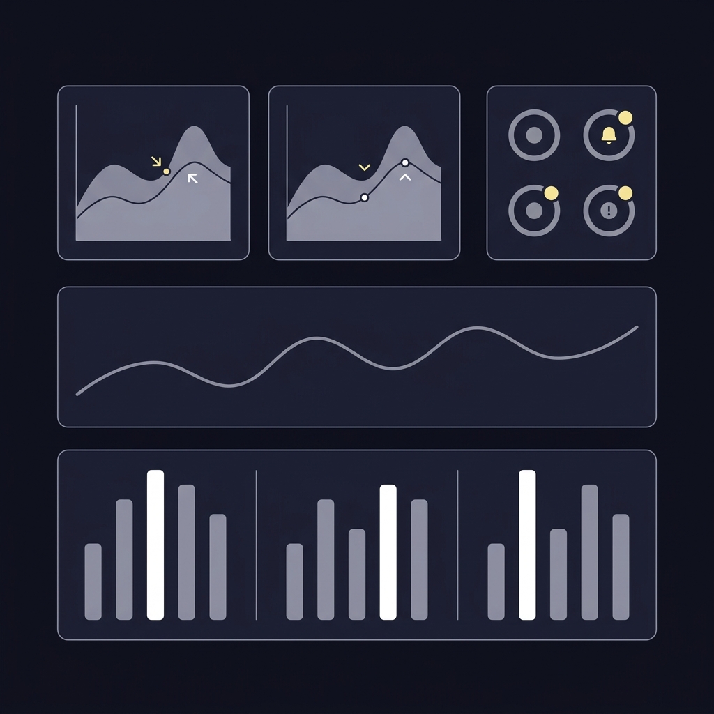
A monitoring dashboard typically tracks per-period metric performance, input feature distributions, and business KPIs. Automate checks that highlight deviations from baseline and configure alerts for breaches of pre-agreed thresholds so that teams can investigate promptly. Make sure monitoring respects the time it takes to observe outcomes and avoids premature reactions to normal variability. For an example of how Funded Plays documents evaluation patterns, see how Funded Plays evaluations work.

Operational responses to alerts can include recalibrating thresholds, retraining on fresh data, pausing the model to investigate, or running a controlled trial to validate corrective actions. The decision should weigh statistical evidence, operational cost, and business risk rather than relying on single-period fluctuations.
Decision criteria: when to trust an edge and when to recalibrate
Trust requires both statistical confidence and economic sensibility. Combine bootstrap confidence intervals, consistency across walk-forward folds, and business-aligned metrics to form a decision rule. A narrow confidence interval that consistently lies above your operational threshold across folds is stronger evidence than a single high point estimate.
When signals conflict, require additional validation such as a fresh out-of-sample test or a controlled live trial before widening deployment. Conservative guardrails include staged rollouts, minimum stability windows, and documented rollback plans to manage downside risk.
Typical mistakes and pitfalls when testing for an edge
Recurring errors that create false confidence include using random k-fold splits on ordered data, tuning on the same data you later call out-of-sample, and choosing metrics that do not match deployment objectives. Each mistake can produce inflated performance that will not survive real-world conditions cross-validation guidance
Other pitfalls are overfitting to calendar events or promotional windows and neglecting to record and freeze the exact pipeline used for evaluation. Simple diagnostics such as re-running the pipeline on a reserved holdout or checking for abrupt metric shifts between adjacent folds catch many of these errors early.
Practical examples and scenarios: applying the framework
Classification validation workflow example: build a pipeline that includes time-aware folds, choose ROC-AUC and Brier score to assess discrimination and calibration, and run bootstrapped intervals across folds to report uncertainty. Summarize per-fold results and document any fold-level failures as part of the release decision. For guidance on metrics and evaluation patterns, standard model evaluation documentation is useful metrics and scoring guidance
Return-oriented scenario: when your outcome is economic, translate predictions into simulated PnL using a plausible execution model, then evaluate mean return alongside a risk-adjusted metric such as Sharpe and check for selection bias using corrections designed for multiple testing. These combined checks help you separate statistical signal from curve-fitting and align performance with business impact the Deflated Sharpe Ratio
When results conflict, for example strong discrimination but weak economic returns, prioritize additional experiments that expose the source of the mismatch: threshold calibration, cost modeling, or a live controlled trial can reveal whether the predictive signal converts to usable advantage.
Checklist and step-by-step workflow to implement in your pipeline
Pre-deployment checklist: construct walk-forward folds that reflect your deployment cadence, reserve a final holdout, select metrics that match decisions, run bootstrap and permutation tests for uncertainty, and capture an audit trail of candidate models and decisions time series cross-validation
Monitoring and response playbook: automate daily or weekly metric checks depending on cadence, monitor feature distributions for drift, set alert thresholds tied to operational KPIs, and define actions for each alert such as retrain, recalibrate, or pause. Ensure that experiment logs, data snapshots, and model artifacts are archived for reproducibility. For additional practical guidance on time-series cross-validation patterns see Time Series Cross-Validation: Practical Guide.
Conclusion: next steps and sustainable practices
Summary of core practices: adopt time-aware validation such as walk-forward folds, choose task-appropriate metrics, quantify uncertainty with bootstrap and permutation techniques, correct for selection bias, and implement continuous monitoring to detect edge decay. These steps together create a disciplined framework for judging whether a model truly has an edge.
Finally, embed these practices into governance and documentation so decisions are reproducible and auditable. See the Funded Plays blog for related posts and governance examples.

Run walk-forward validation at a cadence that matches how quickly the underlying problem changes; slower-changing domains use larger windows and less frequent updates, while fast-moving settings require shorter windows and more frequent retraining.
Use bootstrap confidence intervals for metric uncertainty and permutation tests to assess whether observed performance exceeds chance, while choosing block or time-respecting variants when temporal dependence exists.
Trust it when the improvement is stable across walk-forward folds, the bootstrap interval lies above your operational threshold, and economic-value checks support the decision.