How to Price Player Props: A Practical, Model-First Workflow

What player props are and why fair pricing matters

Definition and common formats, How to Price Player Props

Player props are single-player outcomes offered as individual markets, typically framed as over or under targets or multi-way lines tied to a player statistic. Common formats include count-based props such as goals, shots on goal, or receptions, and quasi-continuous props such as fantasy points, rushing yards, or minutes played. These markets let analysts focus on one predictable element of a game rather than full-game spreads or totals.

To evaluate any single player prop you must start by reading the market price as an implied probability, because quoted odds embed the market's view of the chance an outcome occurs; implied probability is the standard conversion used to turn odds into a base estimate for fair pricing Investopedia implied probability.

Market prices are not neutral measures of chance, because bookmakers include a margin that inflates implied probabilities so the prices sum to more than 100 percent. That margin, commonly called vigorish or overround, is why the next step in fair pricing is removing the bookmaker margin to reveal the market's de-biased probabilities Investopedia vigorish.

A short example helps anchor the idea. If a two-way player prop market shows odds implying probabilities that add to 107 percent, the extra seven percent is the bookmaker margin. De-vigging rescales both side probabilities so they sum to 100 percent, producing a fairer baseline to compare against model outputs.

The step-by-step pricing framework

Overview of the workflow

The practical sequence used by modern analysts can be expressed as four core steps: convert market odds to implied probability, remove margin to obtain de-vigged market probabilities, model the prop to estimate a fair probability, then convert your fair probability back to decimal or American odds for easy comparison and action. Treat this as a checklist you always run before deciding if a price looks like value.

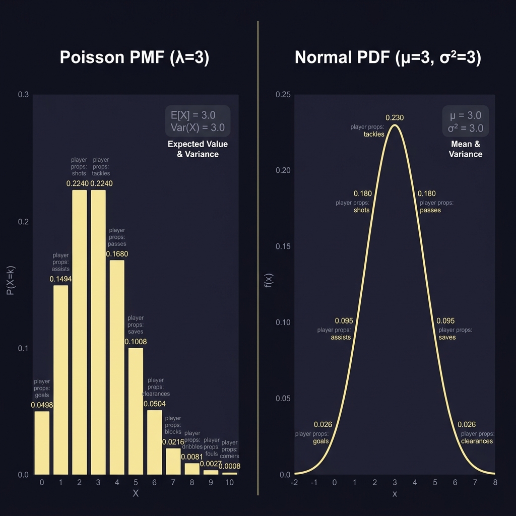
Step 1: Odds to implied probability. Convert the market odds into implied probability using standard formulae that match the odds format on offer. Step 2: Remove margin. Use normalization or another de-vig method to rescale probabilities to a sum of one. Step 3: Model probability. Use a Poisson-family model for count props or a normal approximation for quasi-continuous props to produce a model probability for the specific line. Step 4: Convert back to odds. Translate a final fair probability into decimal or American odds so you can compare on the market's terms and decide whether an edge exists.

When to rely on market prices versus your model deserves attention. The market view can encode information you do not have, such as late news or consensus expectations, while your model preserves your private signal and structural assumptions. Use de-vigged market probabilities as a sanity check and the model probability as your primary estimate when you have reliable inputs and variance estimates.

When to use market prices versus model probabilities

Market prices are useful when liquidity is high and public information moves quickly, but remember that quoted odds include the bookmaker margin and need de-vigging to be comparable to model outputs Pinnacle explainers on betting margins.

Model-derived probabilities are preferable when your data, playing-time estimates, and matchup adjustments capture information not reflected in the market. The choice between trusting the market or your model should depend on the quality of your inputs, recent news flow, and whether the prop is thinly traded.

How to remove the bookmaker margin (vig) and compute fair probabilities

What vig and overround mean in practice

Vigorish or overround is the excess probability baked into quoted odds that lets a bookmaker expect a long-run margin. Practically, overround is the sum of implied probabilities across all outcomes minus one, and it is why raw implied probabilities cannot be used directly as fair prices Investopedia vigorish.

A basic normalization method and alternatives

The simplest and most common de-vig approach is normalization. The recipe is: compute implied probabilities for every outcome in the market, sum those probabilities to get the book total, then divide each implied probability by the book total to rescale the vector so it sums to one. This produces the de-vigged market probabilities that you can compare directly to model probabilities Pinnacle betting margins article. See a no-vig calculator like OddsJam no-vig calculator for quick checks.

Worked numeric example of normalization. Suppose three outcomes show implied probabilities of 0.40, 0.35, and 0.32, which sum to 1.07. The normalized probabilities are 0.40/1.07, 0.35/1.07, and 0.32/1.07, yielding values that sum to 1 and represent the fair market baseline after removing the bookmaker margin.

Alternatives to simple normalization include proportional margin allocation and power methods that attempt to estimate side-specific margins. Those approaches can be useful with asymmetric books or when you have reason to believe the bookmaker's margin is allocated unevenly across outcomes, but normalization is a robust starting point for most player props.

Modeling player props: Poisson for counts and normal approximations for continuous props

When to use Poisson-family models

Count-based player props that record discrete events, such as goals, assists, or shots, are frequently modeled with Poisson-family distributions because these models describe the probability of integer counts occurring over a fixed opportunity set. The Poisson family remains a practical foundation for player-level count props, particularly when event arrivals are reasonably independent and rare within a game window NIST Poisson distribution page.

At player level you often adjust the baseline Poisson rate to account for playing time, teammate influence, and role. For example, an expected goals rate for a forward should scale with minutes and shooting share. When counts are influenced by additional variability, consider negative binomial or mixture extensions to capture extra dispersion beyond pure Poisson assumptions.

Using mean and variance plus the normal CDF for continuous props

Quasi-continuous props such as fantasy points, rushing yards, or minutes played are commonly addressed with a normal approximation: project a mean and a standard deviation, then use the normal cumulative distribution function to convert those moments into the probability a line is exceeded. The normal CDF method is a standard tool for translating a projected mean and variance into over or under probabilities NIST normal distribution guide.

A plain-English conversion looks like this: estimate the prop mean and sd, compute a z-score for the target line as (target minus mean) divided by sd, then read the over probability as one minus the normal CDF at that z-score. This yields a model probability you can compare with the de-vigged market probability.

Be cautious on the edges. Normal approximations work well when the distribution is approximately symmetric and there are enough contributing events, but they can misstate tail probabilities for highly skewed stats or for lines near zero. In those cases, use simulation or a distribution that captures skewness.

Adjustments and edge cases: minutes, usage, matchup and correlation effects

Adjusting models for playing time and role

Playing time and usage rates are primary drivers of player-level expectations. A per-36 or per-100-play baseline is useful for standardizing output, but the final model should scale the baseline by a minutes forecast and adjust for usage changes, such as a larger offensive share when a teammate is injured.

When projecting minutes, build a range of scenarios rather than a single point estimate: starter minutes, reduced minutes, and blowout substitution patterns. Convert each minutes scenario into a probability-weighted outcome so the final model probability reflects both the chance of each minute outcome and the conditional production given that time.

Handling correlations and multi-event props

Correlation matters when a player prop depends on a teammate or team-level event. For example, a quarterback's passing yards prop correlates with team run rate and red zone opportunities. Ignoring correlation can bias your fair price, so include scenario-based adjustments or joint distributions when outcomes are linked.

Funded Plays Challenges

View Challenges

For events with strong dependency, a practical approach is to simulate game-level outcomes that generate consistent joint samples for player stats. That preserves correlation structure and feeds more accurate marginal probabilities than treating each prop independently.

When news alters the tree of scenarios, such as an unexpected injury, widen your variance and rerun the scenario set rather than relying on a single mean. Scenario analysis is often the fastest way to reflect event-driven changes that simple moment-based models miss.

Decision criteria: when a market price looks like value

Edge thresholds and expected value thinking

Define edge as your model probability minus the de-vigged market probability. Expressed relative to the market probability, percent edge helps communicate how much the market would have to be wrong for an action to be profitable in expectation. This simple metric ties model outputs to expected value reasoning.

Set conservative edge thresholds to account for model error, event noise, and market friction. A common practical threshold is to require a material edge before taking a position, and to increase the required edge for less liquid markets or for props with high variance.

Sizing considerations and risk management

Position sizing should reflect both edge and confidence. Use a fraction of your working stake scaled to the perceived reliability of the model and to available liquidity. For props where your model has higher variance or lower sample support, reduce size accordingly to avoid outsized losses from high-variance outcomes.

Keep a running log of bets and model inputs so you can measure realized edge and adjust thresholds over time. Recording assumptions makes it easier to refine your model and reduces the chance of repeatedly acting on systematic misestimates.

Common mistakes and pitfalls to avoid when pricing props

Not removing vig or misreading implied probabilities

Failing to de-vig is one of the most common and costly mistakes because raw implied probabilities overstate the market chance of outcomes, producing apparent edges that vanish after normalization. Always compare your model probability to the de-vigged market probability rather than to raw implied probabilities Investopedia vigorish.

Another frequent error is misreading odds formats or mis-converting between American and decimal odds. Use standard conversion formulas and double-check arithmetic to avoid accidental mispricing when you convert probabilities to odds Investopedia American odds conversion.

Underestimating variance and overfitting models

Relying on mean-only forecasts without sensible variance estimates produces overconfident probabilities that understate tail risk. Where possible, estimate variance from historical residuals or use a conservative floor on sd when sample sizes are small NIST normal distribution guide.

Overfitting to small samples is another frequent pitfall. Resist the temptation to tune many parameters to a short run of results; prefer simpler models that generalize better, and validate with out-of-sample checks or cross-validation where feasible.

Worked example calculations: single-player goals and fantasy points

Example 1: pricing a goals over for a forward using Poisson

Step 1, the market: suppose a goals-over 0.5 line for a forward is quoted at decimal 1.80 for the over and 2.00 for the under, which correspond to implied probabilities. Convert each decimal odd to implied probability by taking 1 divided by the decimal odd, producing a starting implied probability for each side that you will then de-vig Investopedia implied probability.

Step 2, de-vig: compute both implied probabilities, sum them to get the book total, then divide each by that sum to obtain the de-vigged market probabilities. These probabilities are the fair-market baseline you compare with your model estimate. For quick checks use a tool such as TheRundown no-vig calculator.

Step 3, model: using a Poisson-family approach, estimate the forward's expected goal rate for the match window. Suppose your rate is 0.35 expected goals for the game. The probability of scoring at least one goal equals one minus the Poisson probability of zero events, calculated as 1 minus e to the negative rate. Use that model probability as your fair estimate for the over 0.5 line NIST Poisson distribution.

Step 4, compare and convert: if your Poisson model gives a probability higher than the de-vigged market probability by a material margin, convert your model probability to decimal odds as 1 divided by the model probability and to American odds via standard formulae to communicate size. Then decide whether the observed edge clears your execution threshold Investopedia American odds conversion.

Example 2: pricing a fantasy points over using a normal approximation

Step 1, the market: imagine a fantasy points over 35.5 is offered at decimal 1.95. Convert the decimal odd to implied probability as the baseline for de-vigging if you plan to compare to market-derived probabilities.

Step 2, model mean and sd: use historical game logs and usage-adjusted projections to set a model mean of 37.0 fantasy points and an sd of 6.0. Compute the z-score for the line as (35.5 minus 37.0) divided by 6.0, then read the over probability as one minus the normal CDF at that z-score to get the model probability NIST normal distribution guide.

Step 3, de-vig and compare: de-vig the market probabilities and subtract the de-vigged market probability from your model probability to compute the percent edge. If the edge meets your threshold, convert the model probability into decimal and American odds and size according to your risk rules.

These worked examples show the full flow from market odds to implied probability, through de-vigging, modeling, and back to odds so you can make a reasoned decision rather than acting on raw quotes.

Tools, calculators and a practical workflow checklist

Essential calculations and where to automate

Automate the routine pieces: odds to implied probability conversions, de-vig normalization, Poisson probability tables, and normal CDF lookups. A small set of spreadsheet formulas or scripted functions will save time and reduce arithmetic errors when you price many props. See a guide on calculating vig and true odds at OddsIndex, and check our blog for related material.

A concise analyst checklist to follow every time

Copy-ready checklist: 1) Record the market odds and convert to implied probability. 2) De-vig the market probabilities with normalization. 3) Select model type and produce a model probability with variance. 4) Convert model probability to odds and compute percent edge. 5) Check news, minutes, and correlations. 6) Size according to confidence and liquidity. 7) Log inputs and outcomes for backtesting.

Make reproducibility part of the workflow by saving model inputs, assumptions, and scenario weights so you can review which edges worked and which did not over time. That discipline separates repeatable analysis from anecdotal success. Read more about Funded Plays evaluations.

Conclusion: applying fair-price discipline to player props

Key takeaways

The repeatable workflow is straightforward: convert odds to implied probability, remove the bookmaker margin, model the prop with an appropriate distributional approach, and convert your fair probability back to odds to measure edge. De-vigging and clear variance estimates are the two practical ingredients that most improve decision quality Pinnacle on margin methods.

Next steps for practice are simple: build the basic calculators, run the two worked examples on live markets, and keep a disciplined log of model inputs and results to support ongoing refinement. Visit the Funded Plays homepage.