How to Identify Your Most Profitable Odds Range, A Practical Method

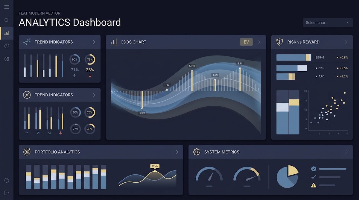
What 'most profitable odds range' means and why it matters

When we say How to Identify Your Most Profitable Odds Range we mean a process that finds the subsets of market odds where your prediction method yields a positive, repeatable edge. In practice this translates to grouping outcomes by odds, computing fair probabilities for those groups, and comparing performance metrics across bands to spot ranges where your model yields better expected returns.

An odds band is simply an interval of prices, for example a 1.20 to 1.50 band or the top 10 percent of implied probabilities. Band-level profitability is typically measured two ways: expected value, which captures the probability-weighted average outcome for a standard stake, and return on investment, which measures net profit relative to total stakes. Both metrics tell different parts of the same story and should be used together when judging a band.

Expected value is useful to assess whether a bet, on average, yields a positive contribution when stakes are normalised, while ROI helps compare how efficient a band is relative to the amount risked. For clarity, many practitioners compute no-vig expected value for a fair baseline, and compute ROI using consistent stake rules so that comparisons are not skewed by varying stake sizes or market liquidity. Expected value definition

Why this matters: market structure and pricing regularities mean different odds ranges can systematically favour or hurt a predictive approach. The favourite-longshot pattern, for example, suggests longshot bands sometimes behave differently than favorite bands, but its strength varies by sport and period. Use careful testing rather than assumptions when you hunt bands.

Preparing your data: odds, outcomes, and no-vig conversion

Start with a minimal, clean dataset: market name, event identifier, runner identifier, decimal odds (record both opening and closing if available), outcome (win or loss), and a stake-equivalent column that encodes the unit stake you will use for aggregation. Having a consistent stake unit is critical because ROI aggregates depend directly on total staked amount.

To compare band-level expected value fairly you must convert decimal odds to implied probabilities and then remove the overround so probabilities sum to one within a market. Converting decimal odds to implied probability is straightforward, then scaling by the market overround yields no-vig probabilities that represent a fair baseline for EV calculations. This no-vig step removes distortions introduced by differing bookmaker margins across markets and is a recommended best practice. Overround explanation

Practical micro-steps, in order: 1) ensure odds are decimal and represent the same book and timepoint, 2) compute implied probability as 1/decimal_odds, 3) compute the market overround as the sum of implied probabilities, 4) obtain no-vig probability by dividing each implied probability by the overround, and 5) persist these transformed fields so every downstream calculation uses the same baseline. Record whether you used opening or closing prices and never mix them without explicit tests, to avoid look-ahead bias.

Defining odds bands: practical segmentation strategies

Choosing sensible band definitions balances resolution against sample size. Fixed-width bands partition the odds axis into regular intervals, quantile-based bins split your data by distribution and guarantee equal sample sizes per band, while market-aware bins group outcomes into operational categories such as favorite, mid-market, and longshot. The right choice depends on your sport, market liquidity, and the analysis goal.

Quantile bins are attractive when sample volume is limited because they avoid tiny counts in specific bands, and fixed-width bands are clearer for reporting and operational rules. Market-aware bins are pragmatic for practitioners who want bands aligned with operational bet sizing or known pricing regimes. When choosing a scheme, version and store the definitions alongside results so your analysis remains reproducible.

As a rule of thumb, avoid bands with fewer than a few hundred independent events when possible, because small samples produce noisy EV and ROI estimates that are hard to trust without strong regularisation or pooling. If your data are thin, prefer coarser segmentation or use rolling-window aggregation to increase effective sample size until out-of-sample validation is feasible.

Calculating band-level metrics: EV and ROI step by step

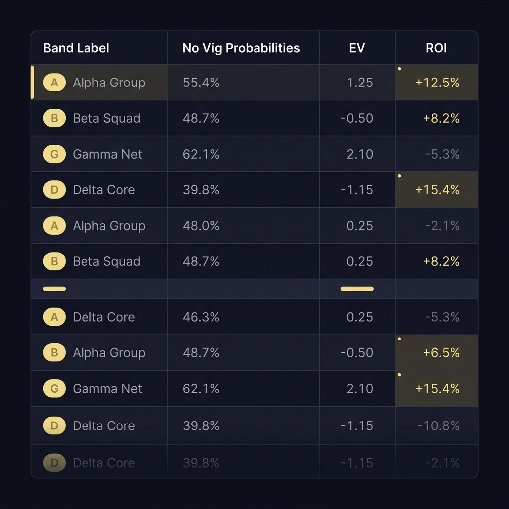
Start with a clear convention for stake sizing. One common approach is to normalise every record to a unit stake, so EV becomes the expected return per unit wagered and ROI equals net profit divided by total units wagered in that band. Using unit stakes makes bands directly comparable regardless of underlying event stakes or market liquidity.

Compute band EV as the average of outcome returns weighted by the no-vig probability that corresponds to the selection, or equivalently as the probability-weighted average of the payoff minus stake for that band. ROI is computed as net profit divided by total stakes within the band. Keep formulas consistent across bands to avoid aggregation artifacts when you later rank or combine bands. ROI reference and formula

Concrete calculation workflow: 1) map each event to a band, 2) use the no-vig probability for expected payout calculations, 3) compute per-event return using the agreed stake convention, 4) for each band sum per-event returns to obtain net profit and sum stakes to obtain total staked, and 5) derive EV and ROI using the defined formulas. Persist intermediate columns such as per-event return and band label to make auditing and debugging simpler.

Quantifying uncertainty: bootstrap confidence intervals for EV and ROI

Statistical estimates without uncertainty are risky to act on. For band-level EV and ROI, nonparametric bootstrap confidence intervals are a robust choice because they do not assume normality and work well with skewed return distributions. The bootstrap approach resamples events within a band, recomputes the metric of interest for each resample, and uses the empirical distribution to form percentile confidence intervals. SciPy bootstrap documentation and a practical tutorial

Funded Plays Challenges page

Explore FundedPlays Challenges

A practical bootstrap recipe: within a band, draw B resamples with replacement (common B values are 1000 or more), compute EV or ROI for each resample, then take the desired percentiles from the resulting distribution to form your confidence interval. If the interval excludes zero you have evidence that the band differs meaningfully from break-even, but interpret results conservatively when samples are small or returns are highly skewed. (See also a UVA library note.)

When you report bootstrap intervals, include the resample count, the percentile method used, and any special handling for tied outcomes or missing fields. These details matter when colleagues reproduce or audit your results, and they help you maintain a transparent living process for band evaluation. See methodological discussions such as an applied bootstrap review.

Controlling false positives: adjusting for multiple band tests

Testing many bands increases the chance of false discoveries. If you evaluate dozens of bands independently, you will likely find some that appear profitable by chance alone. Controlling the false discovery rate helps limit the expected proportion of false positives among bands declared significant, which is often more appropriate for exploratory band hunting than stricter family-wise error control.

Apply a procedure such as Benjamini-Hochberg to the p-values you compute across bands to control the false discovery rate, then report adjusted p-values alongside bootstrap confidence intervals and estimated effect sizes so decision makers see both the magnitude and the adjusted evidence. This combination reduces the risk of acting on spurious bands while still allowing discovery. statsmodels multiple testing reference

A quick practical note: when p-values are not easily available because your inference is bootstrap based, compute bootstrap-derived p-values or use permutation tests, then apply the Benjamini-Hochberg adjustment to those p-values. Always document the method you used to derive p-values so results remain interpretable later.

Practical workflow: building a living odds-band table and dashboard

A repeatable pipeline is essential for staying on top of band-level performance. The living table should ingest raw odds, perform the no-vig transform, assign bands, compute EV and ROI, run bootstrap CI generation, apply multiple-testing correction, and then rank bands by chosen criteria for review. Keep raw and derived fields in the same record to aid audits.

Automation tips include scheduled data pulls from your source, scripted recomputation of transforms and metrics, and a change log that records when band definitions or stake conventions change (see our blogs). Treat band definitions as versioned configuration so historical comparisons remain valid when you update segmentation rules. EV reference

Ranked odds-band table that lists band label, EV, ROI, CI lower and upper bounds, adjusted p-value, sample size, and notes on liquidity or rule exceptions. Use this table during weekly reviews to decide whether a band moves from exploratory status to operational consideration, but only after it survives out-of-sample checks.

Decision criteria: when a band is actionable versus exploratory

Actionable bands should meet a mix of statistical and operational thresholds. A typical rule template combines effect size and confidence with multiplicity control, for example: EV or ROI exceeding a pre-defined threshold, bootstrap CI excluding zero, and an FDR-adjusted p-value below your chosen alpha. These conditions together reduce the chance of committing to a spurious edge.

Adjust thresholds by business constraints. If you have high volume, stricter cutoffs reduce false positives. For low-volume strategies you may accept larger uncertainty but then enforce tighter out-of-sample validation before increasing exposure. Whatever you choose, write the rule down and avoid moving thresholds after seeing results, which invites overfitting. Bootstrap guidance

Operationally, translate an actionable band into conservative entry rules: limit initial stake size, cap exposure per day, and monitor real-time performance. Treat the first weeks of deployment as a probationary period and be ready to revert changes if out-of-sample metrics diverge from in-sample expectations.

Out-of-sample validation and monitoring band stability

Validation prevents look-ahead bias and assesses whether discovered edges hold beyond the discovery sample. Use time-based holdouts, rolling windows, or forward-chaining splits to measure band-level performance on data that was not used to define the bands or tune thresholds.

Track stability metrics such as changes in EV or ROI between periods, CI width, and sign flips that indicate regime shifts. If a band flips sign or its CI widens dramatically, treat the band as suspect until further data clarifies the cause. Re-run multiple-testing corrections and bootstrap procedures on the holdout set before declaring a band operational. Review on favourite-longshot bias

Set a monitoring cadence that fits your volume. High-frequency markets may require weekly checks, while lower-volume sports might suffice with monthly reviews. Always log snapshots of the ranked table so you can trace when and why a band moved between exploratory and actionable lists.

Common pitfalls and how to avoid them

Data leakage and look-ahead bias are perhaps the most damaging mistakes. Using closing-line information, late odds adjustments, or any data informed by the observed outcome will inflate apparent performance. Keep a strict separation between the data used for discovery and data used for validation, and document the exact timepoint for odds you use in analysis.

Small-sample illusions are another frequent trap. Bands with a few wins can look compelling but often fail out of sample. Use bootstrap CIs and FDR adjustments to temper enthusiasm, and prefer coarser bins or pooled estimates when data are thin. Also watch for shifting bookmaker margins which change no-vig baselines over time and can bias band comparisons if not accounted for. Overround reference

Operational mistakes include inconsistent staking and ignoring liquidity constraints. If you mix stake conventions across events, ROI comparisons are meaningless. Similarly, a band that looks good on paper but contains many unbettable lines due to low liquidity is not operationally useful. Keep an eye on sample context and practical execution constraints.

Examples: scenario walkthroughs to find profitable bands

Scenario A, a high-volume soccer market with many draws: here you might prefer quantile bins to ensure sufficient sample size in each band, and you should keep draw probability as a separate outcome type so band assignment handles three-way markets consistently. The banding choice matters because the draw outcome alters return distributions differently than two-way markets, and liquidity concentrated around popular fixtures can skew band samples. (See how Funded Plays evaluations work.)

In Scenario B, a lower-volume NBA market with favorites dominating, fixed-width bands that separate clear favorite zones from mid-market and longshot zones may be preferable. Because sample counts are smaller, you should prioritise coarser bins, rely on bootstrap CIs for uncertainty estimation, and impose stricter out-of-sample tests before operationalising a band. In both scenarios make no claims about guaranteed returns, treat findings as conditional on your data, and validate before scaling exposure. Behavioural insights on favourite-longshot patterns

How pricing biases like the favourite-longshot effect change band expectations

The favourite-longshot bias suggests that the market prices favorites and longshots differently, which can cause band-level expected values to vary systematically. This means longshot bands may show different average mispricing characteristics than favorite bands, but effects vary by sport, market, and era, so you should not assume the bias holds for your dataset without testing.

When you detect signs of the bias, adapt your band rules by testing separate banding schemes for favorites and longshots, and validate whether edges survive out of sample. Do not rely on the bias alone to pick bands; combine bias awareness with the bootstrap and FDR steps to ensure robustness. Journal review of the bias

Summary and next steps: monitoring, updating bands, and responsible participation

Checklist to take away: convert odds to no-vig probabilities, compute band-level EV and ROI with consistent stake conventions, generate bootstrap confidence intervals, adjust for multiple testing, and validate findings out of sample before operational use. Keep band definitions versioned and document every change.

Responsible monitoring means conservative deployment, capped exposure for newly operational bands, and periodic re-evaluation. Results depend on your data, volume, and discipline, and there are no guaranteed outcomes. Treat this process as an ongoing measurement and refinement loop rather than a one-time discovery.