How to Compare Projection Models with Prop Lines: A practical workflow

How to Compare Projection Models with Prop Lines: what this guide covers

How to Compare Projection Models with Prop Lines is a practical, step-by-step workflow that helps analysts align model outputs with market prop lines so they can evaluate accuracy, calibration, and potential edges. The guide focuses on reproducible steps: prepare market data, convert odds to fair probabilities, select point and probabilistic metrics, run out-of-sample tests, visualize diagnostics, and use results to set conservative weighting or threshold rules.

The roadmap below shows the core steps and the intended outcome for each stage. Read straight through for the full workflow or jump to the sections you need.

Roadmap: prepare market data and remove vig, compute MAE and RMSE for point forecasts, score probabilistic outputs with proper scoring rules, calculate closing line value as a market baseline, use out-of-sample tests and visual diagnostics, then choose weighting, ensembling, and stake rules.

Terms used here: prop lines are market prices or totals; projection models produce point or probability forecasts; out-of-sample testing evaluates generalization rather than fit to historical data.

Define projection models and sportsbook prop lines: scope and terminology

Projection models can output simple point forecasts, for example an expected number of points for a player, or full probability distributions that give the chance of outcomes like over or under a given line. Point forecasts are useful when you need a single expected value, while probability forecasts are required when you want to compare model-implied chances to market prices.

Sportsbook prop lines are market prices or posted totals; they are commonly expressed in decimal, fractional, or American odds and reflect both probability assessments and a bookmaker margin. Because market prices include a vig or overround, they do not equal fair probabilities unless that margin is removed, so direct comparisons require conversion and adjustment. For a practical guide to converting odds and understanding the vig, see Pinnacle's explanation of odds conversion and vig removal at Pinnacle betting resources or tools like Unabated's no-vig calculator.

Preparing market data: converting odds into no-vig implied probabilities

Step 1: collect the prop line and its posted odds for each side or outcome, noting the odds format and the timestamp.

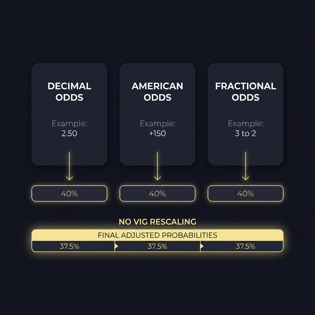
Step 2: convert posted odds to implied probabilities. For decimal odds p = 1 / decimal. For American odds, use p = positive? 100/(odds+100) for + odds and p = -odds/(-odds+100) for negative odds, then normalize. For fractional odds, p = denominator / (numerator + denominator) after converting to decimal. These conversions give raw implied probabilities before removing the bookmaker margin.

Step 3: compute the overround by summing the raw implied probabilities for all mutually exclusive outcomes and dividing each probability by that sum to obtain no-vig probabilities. The no-vig adjustment rescales the market probabilities so they sum to one and provides a fair baseline for comparison. Practical caveats: different books may post different lines at different times, so prefer consolidated snapshots or closing prices when available for robust baselines. For a stepwise explanation of converting odds and removing vig see Pinnacle's tutorial on implied probability and vig removal at Pinnacle betting resources or try a no-vig calculator such as OddsJam's no-vig fair odds tool.

Example calculation: imagine a player points prop where the market posts decimal odds of 1.90 for over and 1.95 for under. Raw implied probabilities are 0.526 and 0.513 respectively, which sum to 1.039. Dividing each by 1.039 yields no-vig probabilities of approximately 0.506 for over and 0.494 for under. Use those no-vig probabilities as the market reference when computing model edges or scoring probabilistic forecasts.

Practical notes: when working with many props, keep timestamps for each odds snapshot and record book identifiers so you can later examine market movement and compute closing line value where possible.

Point accuracy metrics: MAE and RMSE and when to use them

Mean absolute error (MAE) and root mean squared error (RMSE) are the standard metrics for point-forecast accuracy. MAE reports the average absolute difference between model forecasts and observed outcomes, giving a linear sense of expected error. RMSE squares errors before averaging and takes a square root, so it penalizes larger errors more strongly than MAE. For practical evaluation of point forecasts, both metrics are useful because they highlight different aspects of error sensitivity, as described in foundational forecasting literature Forecast accuracy measures.

How to compute and report them: calculate MAE and RMSE across your test sample, report sample averages, and, when possible, provide confidence intervals or bootstrapped estimates to communicate uncertainty. If your error distribution has outliers or heavy tails, RMSE will increase more than MAE and signal that occasional large misses drive performance differences. Use MAE when you want a robust average error and RMSE when large misses are especially costly to your decision process.

Evaluating probabilistic forecasts: proper scoring rules and calibration

Proper scoring rules, such as the Brier score and log loss, reward probabilistic forecasts that are close to observed outcomes and discourage overconfidence. The Brier score measures squared error for probability forecasts of binary events, while log loss (also called negative log likelihood) penalizes confident but wrong predictions more severely. Using proper scoring rules ensures you can compare probabilistic outputs on a consistent, decision-relevant scale; foundational discussion of scoring rules and estimation is available in the statistical literature Strictly proper scoring rules, prediction, and estimation.

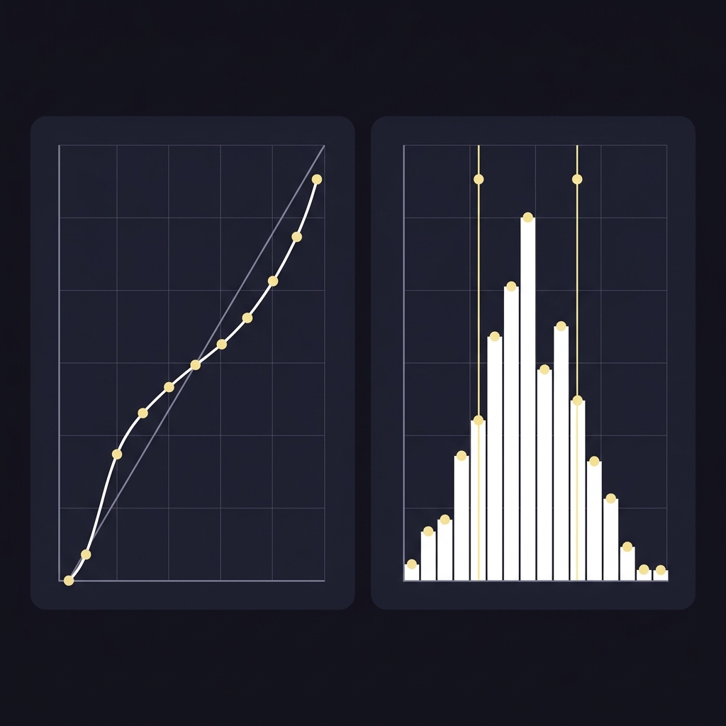
Calibration is the visual and numeric check that predicted probabilities align with observed frequencies. A reliability diagram plots predicted probability bins on the x axis and observed outcome frequency on the y axis; points on the diagonal indicate good calibration, while systematic deviations reveal over- or under-confidence. When miscalibration is apparent, consider recalibration techniques or simple parametric shifts to bring model outputs closer to observed frequencies, especially before converting probabilities into stakeable edges.

Market baselines: no-vig lines, closing line value (CLV), and sample considerations

Closing line value, or CLV, measures how your entry price compares to the final market price and serves as a practical proxy for market efficiency and model quality. Compute CLV per bet as the model-implied edge at the time you posted relative to the closing no-vig probability or closing line; positive average CLV over a large sample suggests your selections priced better than final consensus, which can indicate an edge in practice. For context on CLV and why practitioners use it, see the educational overview of closing line value at Pinnacle article on CLV.

Funded Plays Challenges

Get the sample no-vig spreadsheet

Sample considerations: CLV results require adequate sample size to be meaningful. Watch for selection biases such as only tracking bets you placed, look-ahead bias from using future information, or biased time-of-day sampling. Prefer closing prices when available because they reflect the final market consensus and reduce time-based noise in CLV calculations.

Out-of-sample testing and formal comparison procedures

Always perform out-of-sample evaluation when comparing projection models. Use time-aware splits such as rolling windows, walk-forward validation, or a holdout period that respects chronology to prevent look-ahead bias and overstated performance. Train-test splits that ignore time ordering are inappropriate for sports time series and can produce over-optimistic results. The need for out-of-sample methods and careful accuracy reporting is discussed in forecasting practice references Forecast accuracy measures.

Formal model comparisons should use proper scoring rules as the measurement basis and, where suitable, apply statistical tests for predictive accuracy differences. These comparisons support defensible weighting decisions when ensembling models or choosing a single winner. Keep experiments simple and reproducible: document the split rules, seeds, performance metrics, and any preprocessing to make comparisons auditable and robust. For reproducible writeups and examples, consider posting workflows and periodic performance audits on the Funded Plays blog to keep records accessible.

Visual diagnostics to diagnose bias and variance: calibration curves and edge distributions

Calibration curves visualize how predicted probabilities map to actual frequencies and reveal systematic bias such as consistent overprediction or underprediction across probability ranges. Construct curves by binning predicted probabilities, computing observed frequencies per bin, and plotting the result against the diagonal. This visual check complements scoring rules because it highlights where a model performs well or poorly across the probability spectrum, as explained in the literature on calibration and modern neural network calibration On calibration of modern neural networks.

Edge distributions compare model edge (model probability minus no-vig market probability) across bets. Plotting histograms or density estimates of edges shows whether your model systematically predicts larger margins on some events and whether the distribution has heavy tails, skew, or many small edges. These diagnostics help you set pragmatic thresholds: for example, require a minimum positive edge plus a margin for uncertainty before flagging an actionable selection.

Deciding between models: weighting, ensembling, and threshold rules

Derive simple weights from out-of-sample scores: normalize inverse error metrics or use softmax on negative scores so better-scoring models get higher weights. For example, compute weights proportional to 1 / MAE (or another loss) across models and normalize to sum to one. Keep weighting schemes transparent and stable: tiny sample fluctuations should not flip weights dramatically.

Ensembling often reduces variance and can improve average performance when models make uncorrelated errors. Simple approaches include weighted averages of point forecasts or pooled probability averages for probabilistic outputs. Choose ensembling when distinct model strengths exist and when out-of-sample validation shows the ensemble outperforms individual models. Set conservative threshold rules for actionable edges, for instance requiring a minimum edge plus a buffer derived from model variance estimates before treating an outcome as stakeable.

Practical staking guidance: using edge and variance to set stake rules

Translate measured edge and model uncertainty into conservative stake rules rather than making prescriptive financial claims. A common principle is to scale exposure by both estimated edge and uncertainty: smaller stakes when edge is uncertain, larger stakes when edge is both positive and stable across samples. Use fixed fractional rules with caps and a drawdown-aware cap to keep exposure bounded and predictable.

Risk controls should include maximum per-event exposure, a portfolio cap on simultaneous active props, and periodic re-evaluation of stake rules as model performance and market conditions change. Remember that staking guidance is operational and sample-dependent, not a guarantee of results; treat stake sizing as risk control and measurement rather than a promise.

Common mistakes and pitfalls when comparing projections to prop lines

Frequent errors include failing to remove the vig before comparing probabilities, introducing look-ahead bias by using later market data during model development, and cherry-picking results that favor a particular model. Small-sample CLV or accuracy claims are unreliable and can mislead decision makers when natural variance is ignored. For practical guidance on odds conversion and vig, consult Pinnacle's educational materials on odds and vig removal at Pinnacle betting resources.

Mitigations: document data provenance, enforce time-aware splits, report sample sizes and confidence intervals, and prefer closing price comparisons to reduce transient noise. Maintain reproducible processing scripts and store snapshoted odds and timestamps to allow later audits and recalculations.

Worked example: step-by-step comparison for a player points prop

Setup: assume a small hypothetical dataset of ten player-game events. For each event collect the model point forecast, the observed points, the market decimal odds for over/under, and the closing odds. Convert market odds to no-vig probabilities as described earlier and compute model-implied probability for the same binary over/under outcome by translating the model point forecast into a probability using a chosen dispersion assumption or distribution mapping.

Compute point metrics: calculate MAE and RMSE across the ten events. For example, if model point errors are [1, -2, 0, 3, -1, 2, -3, 0, 1, -1], compute MAE as the mean of absolute errors and RMSE as the square root of the mean squared errors to show sensitivity to the few larger misses. Use the forecasting accuracy discussion as a reference for interpreting these numbers Forecast accuracy measures.

Compute probabilistic scores and CLV: translate each model forecast into a probability and compute the Brier score or log loss for the ten events. Also compute per-event CLV as the difference between model-implied edge at posting and the no-vig closing market edge; average CLV across events to check whether the model consistently outperformed closing markets. For CLV background see the practical explanation at Pinnacle article on CLV.

Interpretation: if MAE is low but CLV is inconsistent, the model may be accurate on average for points but not consistently better than the market on pricing. If calibration plots show overconfidence where high predicted probabilities occur more often than realized, consider recalibration before using probabilities for staking rules.

Interpreting outcomes: what sustained CLV and calibration patterns tell you

Sustained positive CLV over a large, stable sample suggests your approach is capturing value relative to the market, but this is not a guarantee of future success and requires robust sample sizes and bias checks. Empirical discussions of CLV caution that small samples or selective reporting can exaggerate apparent advantages Pinnacle article on CLV.

Chronic miscalibration points to model issues: persistent bias suggests an offset problem, while underdispersion (probabilities too concentrated) indicates the model underestimates uncertainty. Common responses include recalibration using isotonic or Platt methods, revisiting feature sets, or adjusting ensemble weights to increase dispersion. Use diagnostic plots and out-of-sample checks to validate any corrective step.

How comparison best-practices fit into funded challenge workflows

In a funded-simulation challenge environment, the same comparison workflow-no-vig conversion, scoring, calibration checks, CLV monitoring, and out-of-sample tests-helps entrants measure consistency and improve decision rules within the rules and constraints of the challenge. Use documented datasets, reproducible scoring scripts, and periodic performance audits to maintain transparent records for performance review.

Keep brand context factual: FundedPlays provides a platform for structured sports prediction challenges using virtual funded accounts and defined rules; applying rigorous comparison practices can help entrants refine strategies, but improved metrics do not guarantee qualification or rewards.

Conclusion: a concise checklist and next steps for improving models

Checklist: 1) convert odds to no-vig probabilities, 2) compute MAE and RMSE for point forecasts, 3) score probabilities with Brier or log loss and plot calibration curves, 4) compute CLV using closing prices when possible, 5) run out-of-sample tests with time-aware splits, 6) use diagnostics to set conservative thresholds and stake rules, and 7) document all data and processing steps for reproducibility. For iterative improvement, track CLV and calibration trends over time and reweight or recalibrate models when justified by out-of-sample evidence.

Next steps: apply this workflow to a recent block of player props, record closing prices, and review diagnostic plots to prioritize model fixes. Keep experiments reproducible and treat staking as a controlled, sample-dependent activity rather than a promise of returns. For guidance on running evaluations under Funded Plays rules see how FundedPlays evaluations work.