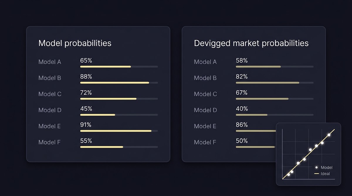
How to Compare Model Output with Market Odds — practical workflow for analysts

How to Compare Model Output with Market Odds: overview and when it matters

Comparing a predictive model to market odds is a core diagnostic for sports analysts and modelers who want to know whether their probability estimates are calibrated and whether any exploitable edge exists. How to Compare Model Output with Market Odds starts from the premise that market prices represent collective information plus a bookmaker margin, so valid comparisons require converting prices to implied probability and removing the margin before computing edge; practical margin calculators and explanations are widely used for this preprocessing step Pinnacle margin calculator.

This article walks through a stepwise workflow you can follow end to end: convert decimal, American or fractional odds into implied probabilities, measure and remove the overround so market probabilities are fair, compute expected value and edge from your model probabilities against those fair prices, evaluate forecast quality with Brier score, log loss and calibration plots, and finally test the statistical significance of observed hit rates and returns. The sequence emphasises reproducibility and out of sample validation so analysts avoid common biases.

How to convert bookmaker odds to implied probabilities and remove the vig

Start by turning quoted odds into implied probabilities using the standard conversions for each format. For decimal odds the implied probability is the reciprocal of the decimal price. For American and fractional formats there are similar conversions to a probability scale. These conversions are elementary but necessary because they place model outputs and market prices on the same probability axis.

Bookmakers typically include a margin so the simple sum of implied probabilities across all mutually exclusive outcomes exceeds one; that excess is the overround or vig. To compare model probabilities to the market fairly you normally remove that margin by normalizing implied probabilities across outcomes, which rescales them so the probabilities sum to one and yield de‑vigged market probabilities. This normalization approach is the standard de‑vig step used in industry guides and help pages Smarkets help on overround.

When markets have many outcomes or correlated lines, normalization is still the default starting point but requires caution; correlated outcomes and live in‑play movements can complicate fair pricing and are active areas of methodological discussion. Use normalization as the baseline preprocessing step and document any deviations when you work with multi‑way or dependent outcome sets.

How to compute expected value and betting edge from model probabilities

Once you have your model probabilities and fair market probabilities you can compute expected value and the betting edge. A common verbal form of the relationship is: edge equals model probability times the fair decimal price minus one. Put differently, expected value per unit stake follows from comparing the model probability to the fair-implied payout, which gives a direct sense of whether the model sees a positive expectation against the market.

Using raw market prices that still include the bookmaker margin biases both the edge estimate and subsequent sizing decisions, because the vig systematically shifts market prices away from fair payouts. That is why de‑vigging must occur before computing edge or feeding prices into a Kelly‑style sizing rule Smarkets help on overround.

For decision rules such as Kelly, always input fair decimal odds rather than raw quoted prices, and be conservative about parameter uncertainty when you translate edge into stake size.

Verification metrics: Brier score, log loss and calibration plots

To judge a probability model you need proper forecast verification. Two widely used scalar metrics are the Brier score and log loss; the Brier score measures mean squared error of probabilities against binary outcomes, while log loss penalizes overconfident, wrong forecasts more heavily. Interpreting these metrics across models and subgroups helps determine whether a model is systematically miscalibrated or simply noisy, and mature implementations are available for practical use NOAA CPC verification methods.

Scalar scores are useful but calibration diagrams, often called reliability diagrams or calibration curves, reveal whether predicted probabilities match observed frequencies across the probability range. A model that is overconfident will lie above or below the diagonal in characteristic ways; visual inspection of calibration plots is an important complement to numerical summaries, and common machine learning libraries include tools to create these plots scikit-learn calibration documentation. See tutorials such as the GeeksforGeeks guide for worked examples.

Funded Plays Challenges

Explore Challenges

In practice you should record both scalar metrics and calibration plots for different bet sizes and market segments. Calibration and score reporting provide an evidence base to decide whether model outputs are reliable enough to feed into an edge-based decision framework.

Testing significance: hit rates, binomial tests and return distributions

When you observe a hit rate or a run of positive returns you need to test whether that performance is unlikely under a null model. For pure hit‑rate questions the exact binomial test is a principled choice: it computes p‑values and confidence intervals assuming independent Bernoulli trials with a given success probability, which is useful when you want to test whether an observed win rate exceeds the fair market probability or some baseline level SciPy binomtest documentation.

Evaluating returns requires distributional thinking. You can use bootstrapping or distributional inference to estimate confidence intervals for average return or cumulative performance, but sports outcomes are often non‑iid and affected by serial dependence or shifting market liquidity. Use out‑of‑sample tests and conservative interpretations, and beware that p‑values alone do not prove long‑term profitability.

Practical toolchain: Python and R libraries for odds conversion, calibration and testing

Implementations for each step of the workflow are available in open‑source toolchains. In Python, scikit‑learn provides calibration utilities and plotting helpers while SciPy supplies exact tests and statistical primitives. In R there are CRAN packages that convert odds formats and helper libraries for plotting and testing, enabling full pipelines from raw prices to evaluation. Kaggle notebooks offer hands-on examples and worked tutorials Kaggle probability calibration tutorial.

To keep analyses reproducible, pin package versions, control random seeds for stochastic steps, and archive notebooks or scripts with environment manifests. These practices reduce accidental variation and make results easier to audit and repeat across teams scikit-learn calibration documentation.

Decision framework: when your model shows an edge and how to act

Deciding when to act on a measured edge blends statistical confidence with operational checks. Set a minimum edge threshold that accounts for transaction costs, liquidity, and model uncertainty, and require supporting evidence such as a favorable calibration in the relevant probability band and a statistically meaningful test result before deploying capital or stakes.

Before placing any stakes, check market liquidity, whether the line remains available at the fair price you measured, platform stake limits, and any rules that govern your participation. Validate your decision with out‑of‑sample performance and treat early deployment as a controlled experiment rather than a proven strategy.

Risk controls and bet-sizing when comparing model output with market odds

Principled sizing uses the best available edge estimate and an honest account of uncertainty. Because Kelly and related formulas convert edge into stake fractions, feeding them de‑vigged fair odds is essential to avoid systematic bias in recommended sizes. When uncertainty or model drift is high, the conservative approach is to use fractional‑Kelly or fixed cap sizes.

Track variance and drawdown limits and treat violations as triggers for a formal review. Maintain stop rules and review cadences so that a sequence of adverse outcomes leads to model reassessment rather than ad hoc doubling of stakes.

Common mistakes and pitfalls when comparing models to market prices

Several procedural errors recur in practice. The most basic is failing to remove the bookmaker margin before computing edge, which biases edge estimates and any downstream sizing rule. Document your de‑vig method and test it on known cases to ensure consistency Pinnacle margin calculator.

Other frequent errors include relying on in‑sample results, overfitting model parameters to historical prices, and ignoring market microstructure effects such as correlated outcomes or in‑play line movement. Each of these can make a promising in‑sample result evaporate when faced with real market conditions.

A step-by-step example scenario: converting lines, computing edge and evaluating results

Outline the ordered steps you would follow for a single market: retrieve quoted prices and timestamps, convert prices to implied probabilities by format, compute the market overround and normalize to obtain fair probabilities, calculate edge as model probability times fair decimal price minus one, and then record evaluation metrics including Brier score and log loss. Log all intermediate values so you can audit any decision later.

For reporting create a standard output row per event containing at minimum: event identifier, timestamp, raw odds, implied probabilities, de‑vigged probabilities, model probability, computed edge, stake recommendation and outcome. Store calibration plot images and the scalar scores for time windows so you can track model stability and performance drift over time NOAA CPC verification methods.

Implementing reproducible pipelines and avoiding overfitting

Use time‑aware splits rather than random shuffles for sports data, and adopt train, validation and test partitions that respect chronological order. Time series cross‑validation techniques help estimate out‑of‑sample performance without leaking future information into model training.

Version control code and dataset manifests, pin package versions in environment files, and save experiment metadata including seeds, parameter snapshots and data retrieval queries. These steps make it feasible to reproduce a reported result months later and to diagnose whether a change in performance stems from data drift or a code change.

Checklist: what to report when you compare model output with market odds

A reproducible report should include data provenance, odds conversion formulas, the de‑vig method used, model probability definitions, evaluation metrics, and the exact statistical tests applied. Include environment details and a link or pointer to the script or notebook that produced the figures so reviewers can rerun the steps. See the Funded Plays blog.

Visuals to include are calibration curves for key probability bands, time series of cumulative returns and a table of per‑segment scalar scores. These outputs together let readers assess whether a measured edge is consistent, robust across segments, and stable over time CRAN odds.converter.

Conclusion: practical next steps and ongoing questions

In summary, a sound workflow first converts odds to implied probabilities, removes the overround to obtain fair market probabilities, computes edge from model probabilities against those fair prices, evaluates forecast quality with appropriate metrics, and tests statistical significance with out‑of‑sample checks. That sequence reduces bias and improves the interpretability of any claimed edge Smarkets help on overround. See how Funded Plays evaluations work.

Open questions remain around market microstructure, correlated outcomes and in‑play line dynamics; treat those as advanced topics to address after you have a reproducible baseline pipeline. Monitor performance continuously and report results transparently; responsible, evidence based iteration is the most reliable path to meaningful conclusions.

Appendix: resources and links for implementations

Key references to implement each step include margin and overround calculators, calibration documentation and statistical testing references. These sources provide both the conceptual background and links to practical implementations you can adapt in Python and R Pinnacle margin calculator. See the Funded Plays homepage.

For calibration and plotting consult the scikit‑learn calibration documentation, and for exact binomial testing consult SciPy's binomtest reference. For odds format conversion in R, the CRAN odds.converter package is a convenient starting point scikit-learn calibration documentation. See the Machine Learning Mastery tutorial on probability calibration here.

Evaluating returns requires distributional thinking. You can use bootstrapping or distributional inference to estimate confidence intervals for average return or cumulative performance, but sports outcomes are often non‑iid and affected by serial dependence or shifting market liquidity. Use out‑of‑sample tests and conservative interpretations, and beware that p‑values alone do not prove long‑term profitability.

For decision rules such as Kelly, always input fair decimal odds rather than raw quoted prices, and be conservative about parameter uncertainty when you translate edge into stake size.

Version control code and dataset manifests, pin package versions in environment files, and save experiment metadata including seeds, parameter snapshots and data retrieval queries. These steps make it feasible to reproduce a reported result months later and to diagnose whether a change in performance stems from data drift or a code change.