How to Analyze Upset Potential: A Practical Workflow

How to Analyze Upset Potential: convert odds into a fair market baseline

What implied probability means and why bookmakers build an overround

The first step in any upset probability analysis is to convert published odds into implied probabilities so you and your model are speaking the same language. Implied probability is the direct transformation of odds into a chance estimate, and it is the foundation for comparing a model to market expectations; for a clear primer on conversion and interpretation see the Smarkets Academy guideSmarkets Academy guide. For quick conversion tools see Covers' odds converter Covers odds converter.

Bookmakers generally publish prices that include an overround, a built-in margin so the raw implied probabilities sum to more than one. That overround means you cannot directly compare raw implied probabilities to your model without first normalizing the book's side margin, because the surplus probability inflates underdog and favorite chances alike; a straightforward explanation of the concept is available on Wikipedia's overround pageWikipedia on overround.

Step-by-step: converting odds to implied probabilities and removing overround

Follow these simple, actionable steps to obtain a fair market baseline you can trust before comparing model outputs. Step 1: convert the posted price to implied probability. For decimal odds the formula is 1 divided by the decimal price. For American odds use the standard conversion rules for positive and negative values. Step 2: sum the raw implied probabilities for all outcomes in the same market to measure the overround. Step 3: divide each raw implied probability by the sum of raw implied probabilities so the normalized probabilities sum to one; the normalized values are the fair market probabilities. This produces a disciplined reference point you can use in upset probability analysis. You can test conversions with tools like OddsJam's implied probability calculator OddsJam implied probability.

Worked numeric example: assume a three-outcome match with decimal prices 3.20, 2.10, and 4.50. The raw implied probabilities are 0.3125, 0.4762, and 0.2222, which sum to 1.0109. Divide each by 1.0109 to remove the overround and produce fair probabilities that sum to one. Using this routine converts messy listed prices into a stable market baseline, which is why closing prices in liquid markets are preferred when building references for underdog evaluation. For a quick calculator try TheRundown's implied probability tool TheRundown calculator.

Keep these practical notes in mind: use consistent odds formats across data sources, apply the same normalization across both pregame and closing markets, and document whether you used early or closing prices. That discipline reduces confusion when you later compute a model-market value gap.

How to Analyze Upset Potential: measure the value gap versus the market

Defining value gap: model probability minus fair market probability

Once you have fair market probabilities, define the value gap as your model's predicted probability minus the fair market probability for the same outcome. A positive value gap suggests your model assigns a higher chance to the underdog than the market does, which flags a possible opportunity; for a practical discussion of value concepts in betting contexts see Pinnacle's discussion of value bettingPinnacle on value betting.

Example: if the normalized market probability for the underdog is 0.22 and your model gives 0.30, the value gap is 0.08. That gap translates into expected value only when combined with a staking or exposure rule that accounts for variance and liquidity.

Why closing market prices are the recommended benchmark in liquid markets

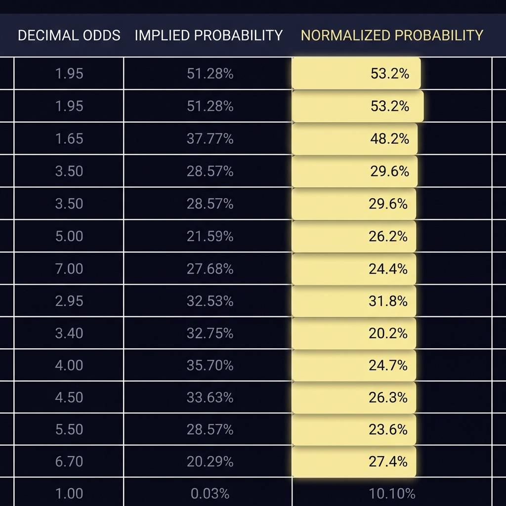
Benchmarking against closing prices is a best practice because, in liquid markets, closing prices tend to incorporate the most information and narrower spreads than early lines. Use closing prices when available for your baseline and track whether market liquidity is sufficient to trust that price as an informationally efficient reference.

Practical note on liquidity: when a market is thin, individual large orders, late news, or correlated events can move prices sharply, producing misleading gaps. In those cases you should widen your internal thresholds for action or require a larger model confidence margin before treating a value gap as actionable.

A small table-style mental checklist helps keep things consistent: column one, model probability; column two, normalized market probability; column three, value gap; column four, liquidity note. Review these for every candidate underdog and avoid overreacting to single-game gaps caused by thin markets or temporary pricing anomalies.

Model evaluation: use proper scoring rules and calibration checks

Why hit rate is insufficient and what strictly proper scoring rules measure

Evaluating an underdog model requires measures that reward honest probability estimates. A raw hit rate or win percentage punishes sensible probabilistic forecasts because it ignores confidence: assigning 51 percent to many events can yield the same hit rate as a risky pattern while being more calibrated. Strictly proper scoring rules, like the Brier score and log loss, are designed to reward calibrated, sharp probability forecasts over time; for the theoretical foundation on proper scoring rules see the classic PNAS treatmentPNAS paper on strictly proper scoring rules.

Use a rolling-window evaluation to track whether the model is improving or degrading against these scoring rules rather than focusing on isolated hit-rate snapshots. That approach gives you a continuous sense of model health and helps detect drift.

How to compute and interpret the Brier score and log loss

The Brier score is the mean squared error between predicted probabilities and realized outcomes (where the realized outcome is 1 for a win and 0 otherwise). Lower Brier scores are better because they indicate predictions are on average closer to outcomes; the Brier score explicitly rewards calibration and sensible confidence levels.

Log loss penalizes overconfident, wrong predictions more heavily than the Brier score and is useful when you want to discourage extreme probability estimates unless they are well justified. Interpret log loss as a measure of how surprised the model is by outcomes on average; smaller values indicate a better probabilistic fit.

Practical computation advice: compute both scores over rolling windows (for example, 30 to 90 games depending on your sport's sample rate), chart them, and flag persistent deterioration. Use these scores to prioritize model revisions when calibration or sharpness declines rather than chasing short-term gains in hit rate.

Verify calibration: reliability diagrams and calibration tests

Constructing a reliability diagram for underdogs

A reliability diagram groups predicted probabilities into bins and compares average predicted probability to the observed frequency of the event in each bin. Plot the average predicted probability on the x-axis and the observed frequency on the y-axis; a well-calibrated model will lie close to the diagonal line. For practical guidance on calibration techniques and plotting, the scikit-learn user guide provides stepwise instructions you can follow in a notebook or spreadsheet environmentscikit-learn calibration guide.

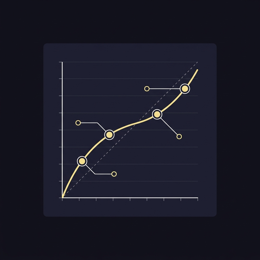
Implementation steps you can do in a spreadsheet: create equal-width probability bins (for example, 0.0 to 0.1, 0.1 to 0.2, and so on), assign each prediction to a bin, compute the mean predicted probability and the empirical outcome frequency for each bin, and plot those pairs. Repeat the diagram for rolling windows to see whether calibration drifts over time.

Interpreting miscalibration and how to correct it

When the reliability diagram shows points above the diagonal, the model is underconfident for those bins, meaning the observed frequency is higher than predicted. When points fall below the diagonal, the model is overconfident and probabilities are too high for the observed frequency. Corrective actions include logistic recalibration, isotonic regression, or simple shrinkage toward market probabilities depending on sample size and the direction of miscalibration.

Use statistical calibration tests and visual inspection in tandem. Visual checks reveal where the model departs from ideal behavior and are easier to communicate to stakeholders; formal tests can quantify evidence of miscalibration but are sensitive to sample size and binning choices. Regularly recompute calibration over season-specific windows to account for structural changes across competitions.

Core frameworks: pairwise rating models and integrating market priors

Overview of Elo and Bradley Terry style pairwise models as transparent baselines

Pairwise rating frameworks such as Elo or Bradley-Terry provide transparent baselines for upset probability analysis because they express relative strength as a rating difference and map that difference to win probabilities. These models are stable, interpretable, and simple to update with game outcomes, making them a good starting point when building an underdog probability baseline; standard pairwise thinking and rating translation remain widely used in practice for this reason.

Keep the implementation simple at first: compute ratings from recent results, translate rating differences into baseline win probabilities with a logistic link, and measure performance with the same scoring rules and calibration checks described earlier. These baselines are easy to explain and serve as a sanity check before introducing many additional covariates.

How to combine a rating-based prior with market-implied probabilities

One practical blending approach is to treat the rating-based probability as a prior and shrink it toward the market-implied probability by a weight that reflects your confidence, recent form, and market liquidity. For example, form a weighted average where the weight on the market increases with liquidity and decreases when your model has demonstrated superior calibration historically.

Include recent-form covariates and short-term interaction terms to capture nonstationary effects like streaks or injuries, then re-evaluate whether the blended forecast improves Brier score and calibration on rolling windows. If the blended forecast consistently outperforms both the raw model and the market baseline on proper scoring rules, it represents a robust upset probability estimate to monitor.

Situational adjustments that matter for upset chances

Home advantage, crowd effects, and how to re-estimate situational priors

Contextual factors such as home advantage and crowd effects can materially shift underdog chances. Evidence from natural experiments during the pandemic suggests home advantage declined notably when crowds were absent, which is a reminder to re-estimate situational priors after structural changes to the environment; for background on probability calibration and related effects, consult calibration and reliability literature as a practical referencescikit-learn calibration guide. For discussion of evaluations see our blog at how fundedplays evaluations work.

When a league rule change, scheduling reform, or other structural event occurs, re-fit the home advantage term with a recent-window estimate rather than assuming historical averages. That reduces the risk of transferring out-of-date situational effects into your underdog probability estimates.

Funded Plays Challenges

Get the worksheet

Rest, travel, schedule density and short-term form effects

Short-term factors such as rest days, travel distance, and schedule density are measurable covariates that often shift upset chances in the short run. Quantify these factors as simple variables in your model (for example, days since last game, cumulative minutes played, travel time buckets) and test their incremental contribution via out-of-sample Brier score improvements.

Be cautious when transferring situational estimates across leagues or seasons. Differences in style, roster depth, and scheduling mean that a rest effect estimated in one competition may not generalize. Validate any situational adjustment with rolling-window tests and document the performance uplift before committing to it in production.

Decision criteria and risk management: when an underdog is worth tracking

Practical thresholds and using expected value concepts

Turn a positive value gap into an operational rule by combining the magnitude of the gap with model confidence and market liquidity. A simple thresholding rule could require a minimum value gap plus a minimum sample-based confidence level from your model before you mark a game for tracking.

Frame decisions with expected value and variance: a modest value gap on a single game yields a small expected return but can have large variance. Use expected value in conjunction with exposure sizing to set limits on drawdown and to maintain consistent risk controls in a funded challenge environment. See related resources on the Funded Plays site at Funded Plays.

Monitoring performance and adjusting bet sizing or exposure in a funded challenge context

Monitor decisions by logging predicted probability, market baseline, value gap, outcome, and the Brier score contribution for each tracked game. Use a rolling evaluation window to adjust sizing rules if realized variance or drawdowns exceed your risk tolerance. In a structured funded challenge, preserve capital-like constraints and avoid concentration on a small set of correlated underdogs.

Prefer conservative, repeatable rules and treat sizing as conditional on model calibration. If calibration degrades, reduce exposure and focus on corrective model work rather than doubling down on an apparent edge that may be an artifact of miscalibration.

Common mistakes and troubleshooting an underdog model

Typical pitfalls: overfitting, ignoring calibration, and chasing hit rate

Common errors include overfitting situational covariates to a limited sample, ignoring calibration, and optimizing for hit rate rather than proper scoring rules. Overfitting often shows up as impressive in-sample accuracy with poor out-of-sample Brier scores and erratic reliability diagrams.

When you see a run of unexpected outcomes, run a compact diagnostic checklist: check rolling-window Brier and log loss, replot the reliability diagram for recent games, test for structural changes in home advantage or schedule effects, and inspect liquidity notes for the markets you acted on. That sequence helps distinguish model decay from simple variance.

How to run diagnostics and when to recalibrate

Recalibrate when rolling-window scoring rules show persistent degradation or when the reliability diagram reveals systematic bias. Use simple recalibration methods initially, such as logistic shrinkage toward market probabilities or isotonic regression when you have a larger sample, and re-evaluate performance on withheld data to confirm improvement.

Maintain a practice of logging diagnostic outcomes and decisions so you can audit when and why you recalibrated. That history prevents repeated overreaction and supports disciplined long-term improvement.

Practical examples and next steps

Worked mini case: spotting an underdog with a positive value gap and checking calibration

Worked mini example: start with listed decimal odds for the underdog, convert to an implied probability, remove the overround, and record the fair market probability. Next, compute your model probability using your baseline rating or machine model. Subtract the fair market probability from your model probability to get the value gap. If the gap exceeds your pre-defined threshold and the market liquidity is acceptable, log the selection for tracking and record the Brier score contribution when the event resolves. See related blog posts at Funded Plays blog.

As you run these checks, verify that the model's recent reliability diagram shows reasonable alignment between predicted probabilities and observed frequencies in the bins relevant to your action threshold. If calibration is off in the action range, either recalibrate or increase the value gap threshold until calibration is restored.

Suggested implementation checklist and monitoring routine

Implementation checklist: 1) collect prices and convert them to implied probabilities, 2) remove the overround and set fair market baselines, 3) generate model probabilities and compute value gaps, 4) apply decision thresholds that include liquidity and confidence checks, 5) log each decision with scoring contributions, and 6) run weekly rolling-window Brier and calibration diagnostics.

Next steps: implement the checklist in a spreadsheet or notebook, test the pipeline on past seasons if possible, and iterate using rolling-window performance feedback. Treat this as an experiment: record hypotheses, test outcomes, and adjustments to maintain an empirical improvement cycle for your upset probability analysis.