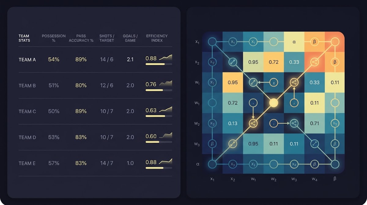
How to Adjust Statistics for Opponent Quality, A Practical Method Guide

How to Adjust Statistics for Opponent Quality: definition and context

Opponent-quality adjustment means converting raw team or player numbers into values that reflect the strength of the opponents those numbers came against. Raw averages, like points per game or yards allowed, mix performance and schedule. That makes direct comparisons misleading when teams or players face very different opponents or spend more time at home or away.

At a simple level, an opponent-adjusted statistic asks, how would this performance look if opponents were average? The adjustment corrects for the fact that a strong defense will naturally lower opponents' scoring, and a weak schedule can inflate counting stats. Team-level adjustments focus on making team efficiencies comparable. Player-level adjustments try to isolate an individual contribution after accounting for teammate quality and the opponents faced.

Public rating systems emphasize this point because prediction depends on comparable inputs. Systems that serve fans, analysts, and selection committees explicitly remove opponent bias to make numbers predictive and fair. For example, major public systems in college sports adjust for opponent strength and game location rather than relying on unadjusted averages, which improves comparability across schedules and venues, as described by the system explanations (DVOA explainer).

Adjustment does not guarantee perfect forecasting. It reduces a major source of bias and improves the stability of comparative metrics, but every method has trade-offs between bias and variance. Expect better comparability and typically improved predictive power, while also validating models with out-of-sample checks before relying on adjusted outputs for decisions.

In practice you will see two related uses: team-level adjustment that normalizes efficiencies and margins, and player-level modeling that separates individual impact from opponent and teammate context. Both matter: team-level adjustments help rank squads for match forecasting, while player-level adjustments are needed when the goal is roster evaluation or lineup decisions.

Terminology to watch for includes opponent-adjusted statistics and strength of schedule adjustment, phrases you will see repeatedly when reading methodology pages and model writeups.

Core frameworks: building strength-of-schedule multipliers from linear ratings

One practical way to normalize team numbers is to compute strength-of-schedule multipliers from a simple linear rating system. The Massey approach shows the idea clearly: treat game results as linear equations connecting team strength values and solve the system to estimate team ratings. Once you have team ratings, you can derive a multiplier that scales raw efficiencies toward what they would be against an average opponent.

The Massey method sets up one equation per game encoding margin and home advantage, then solves the resulting linear system for team strength estimates. That produces an interpretable rating for each team and a straightforward path to a strength-of-schedule factor that weights opponent ratings by schedule frequency. For a practitioner, the computation is a solve of a matrix equation built from game outcomes.

Colley offers a complementary, bias-minimizing route. It constructs a win-loss matrix and a regularized set of equations that produce rankings without relying on margin information. The Colley approach yields a bias-free estimate of team quality that can be converted into an SOS measure by aggregating opponents' Colley ratings across the season.

To apply either approach to raw averages, compute the ratio of expected performance versus average-opponent performance. For example, if a team’s rating implies they face opponents 8 percent weaker than average on offense, scale the team’s offensive efficiency upward by the inverse of that factor to estimate an average-opponent baseline. That multiplier approach is computationally cheap and easy to explain to stakeholders.

Pros and cons are clear. SOS multipliers are quick, transparent, and useful for team normalization, but they lack the fine-grain control needed to isolate player effects or account for lineup-level matchups. For player-level isolation you will later combine these multipliers with regression techniques to reduce confounding from teammate and opponent selection.

For readers who want to try a quick sketch, the steps are: build a game matrix, solve for team ratings with a linear solver, compute each team’s average opponent rating, then form a multiplier as average rating divided by opponent average. This rough pseudocode captures the flow without deep linear algebra work.

Regression approaches: regularized adjusted plus-minus and partial pooling

Adjusted plus-minus estimates a player or unit effect while holding constant the other players and the opponent. Naive adjusted plus-minus is noisy because playing time is uneven and lineups correlate. Regularization, usually ridge regression, shrinks noisy coefficients toward zero and produces more stable estimates. This version, often called regularized adjusted plus-minus or RAPM, is a practical standard for player isolation.

In RAPM, opponents and teammates are encoded as covariates in a regression framework. The model assigns coefficients to each player and may include team or game-level covariates for opponent strength and site effects. Regularization limits coefficient spread, which reduces overfitting and improves out-of-sample performance, especially with limited lineup diversity.

Partial pooling alternatives, such as hierarchical models, share information across players or units, letting weak samples borrow strength from the group mean. That reduces variance for players with little data and preserves meaningful differences for well-sampled players. Cross-validation and out-of-sample testing are essential to set regularization strength and confirm that estimates generalize.

Practical implementation requires play- or possession-level indicators that map actions to the relevant on-court or on-field participants, plus enough lineup variation to separate effects. Compute a holdout error metric, tune the ridge penalty with cross-validation, and check coefficient stability across seasons or splits to detect overfitting before deploying player-level adjustments.

Computationally, RAPM is accessible with standard linear algebra libraries and can handle large design matrices if you use sparse representations and a scalable solver. The approach has been shown to improve out-of-sample stability when isolating player impact while controlling for opponent and teammate quality.

Play-level and possession models: benchmarking by situation and opponent

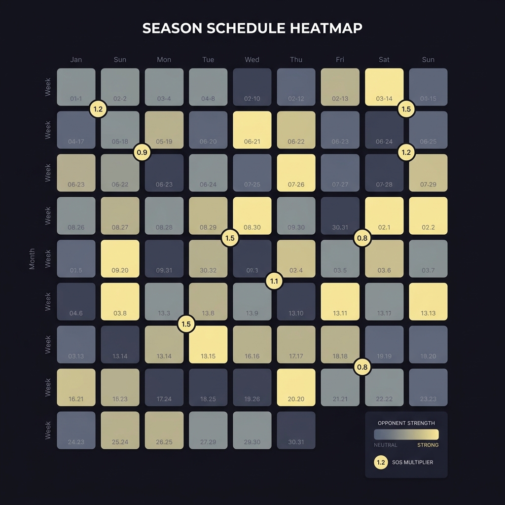
Play-level models refine opponent adjustment by evaluating each play or possession against a baseline conditioned on situation and opponent context. Instead of asking how a team performed per game, these models ask how a play performed relative to expectation given down, distance, field position, game clock, and opponent tendencies.

One well-known example benchmarks play outcomes versus opponent-conditioned baselines to produce an efficiency measure that is naturally opponent-adjusted. That idea underpins approaches used in common efficiency metrics and is core to systems that compare play outcomes to what a neutral baseline would expect (Evaluating NFL Plays).

For football or basketball this means different data granularity. Football models often operate at the play level with down and distance features, while basketball models operate on possessions and account for pace and touch location. Play-level benchmarking typically requires detailed play-by-play feeds and careful feature engineering to capture game state cleanly.

When you build a possession-level model, you condition expected outcomes on situational features and on the opponent’s historical behavior. A short pass on third down has a different baseline expectation against a top defensive team than against a weaker unit, and the model measures value added relative to that opponent-conditioned baseline.

Play-level benchmarking typically requires detailed play-by-play feeds and careful feature engineering to capture game state cleanly. See approaches that adjust EPA for opponent strength (Adjusting EPA for Strength of Opponent).

Data needs are higher for play-level models, but so are potential gains. Possession or play models can surface opponent-specific strengths and weaknesses that team-level averages mask. When play-by-play data is available and you need matchup-level insights, the added complexity is frequently worthwhile and can materially improve prediction in short-term forecasting tasks.

Practical workflow: combining SOS multipliers with shrinkage regression

Combine the speed of SOS multipliers with the isolating power of shrinkage regression to balance bias and variance. A practical pipeline moves from data ingestion to a two-stage adjustment that is straightforward to implement and validate in production.

Stage one, compute SOS multipliers from a linear rating or win-loss matrix and use them to normalize team-level efficiencies as quick baselines. Many public systems blend opponent strength and site effects when producing adjusted efficiency components, and adopting an SOS-based first pass mirrors that effective, low-latency practice.

Stage two, feed normalized efficiencies and lineup indicators into a regularized regression that includes opponent and site covariates to isolate player or unit effects. Regularization and partial pooling stabilize coefficients for players with sparse minutes and help control for collinearity introduced by stable lineups or uneven scheduling.

Operationally the pipeline looks like this: 1) ingest schedules, box scores, and play logs, 2) compute SOS multipliers with a Massey or Colley solver, 3) apply multipliers to team efficiencies, 4) build a design matrix for RAPM with opponent and site covariates, 5) train with ridge or hierarchical shrinkage, 6) validate using holdout splits, and 7) update opponent priors on a regular cadence as the season progresses.

One practical recommendation is to update opponent strengths frequently early in the season with higher shrinkage, then reduce shrinkage as sample sizes grow. That blends a prior belief about team quality with fast-moving evidence from new games, preventing overreaction to small samples while allowing the model to track real change.

Funded Plays Challenges

Explore Funded Plays Challenges

For organizations or analysts who want a simulation sandbox to test pipelines, a funded challenge style environment offers a safe place to validate methods and measure skill without real-money exposure. Platforms that host structured prediction challenges let you run the full ingestion, adjustment, and validation loop while comparing results to public-system baselines. (See Funded Plays.)

Include home/away or neutral-site indicators as additive covariates in the regression stage. Modern public systems commonly include location effects alongside opponent strength, and treating site as an explicit variable provides an easy, interpretable correction that improves predictive accuracy for match-level forecasts. (See our blog for related writeups.)

Decision criteria: choosing between multipliers, regression, and play-level models

Which approach to use depends on data, goals, and resources. Use SOS multipliers when samples are small, you need quick normalization, or computational constraints preclude large regressions. Multipliers are interpretable and give immediate schedule-aware adjustments for team-level analyses.

Move to regression-based methods like RAPM when you have sufficient variety in lineups and enough observations to separate effects. When the goal is player isolation, lineup-level regression with shrinkage typically outperforms multiplier-only approaches at predicting future individual contributions.

Choose play-level models when play-by-play data is available and you need situationally aware predictions. If matchup nuances and situational decision value matter to your forecast, the extra engineering and data cost can be justified by improved short-term predictions.

Also weigh latency. Multipliers can be recalculated quickly each day, while RAPM-style regressions and play-level recalibrations may be batched weekly. Resource and latency trade-offs matter when you plan live updates. Finally, always include site effects as part of your decision matrix, since home, away, and neutral contexts shift baseline expectations consistently across sports.

Common mistakes and pitfalls when adjusting for opponent quality

One frequent error is double-counting adjustments, such as applying multiple overlapping opponent corrections that together overcompensate for schedule differences. Another mistake is failing to shrink noisy estimates, which leads to overfitting when samples are small.

Ignoring pace, site, or opponent style creates bias. For instance, a team that runs a slow pace will show lower counting stats without being worse. Always check pace and context before attributing differences solely to opponent quality.

Short fixes include: use shrinkage regression to control variance, run cross-validation, and sanity-check outputs against public systems. Public systems provide a useful baseline for sanity checks because they incorporate opponent and site adjustments widely accepted in the community.

Another common pitfall is assuming an adjustment is neutral across time. Early-season SOS estimates are noisy; increase shrinkage early and relax it as seasons unfold. Always test on holdout data to ensure your adjustments improve, rather than hurt, out-of-sample forecasts.

Practical examples and scenarios: from team normalization to player RAPM

Worked example, team normalization. Suppose a college basketball team posts an offensive efficiency of 1.08 points per possession but its opponents are collectively 6 percent weaker than average by your SOS ratings. To normalize, divide by 0.94 to estimate what the offense would look like against an average schedule, producing an adjusted efficiency near 1.149. This simple multiplier shows how schedule can materially shift apparent performance.

Include a location adjustment by adding a site factor before dividing by opponent strength. If the team enjoyed an unusual number of home games and your site model estimates home advantage at 3 percent, incorporate that as an additive or multiplicative correction depending on your multiplier convention, and then apply the SOS scaling.

Worked example, player RAPM. Collect lineup data, minutes, and box contributions for the season. Build a sparse design matrix with indicator columns for each player on court, plus opponent and site covariates. Fit a ridge regression, tune the penalty by cross-validation, and interpret a player coefficient as the expected difference in points per possession attributable to that player after controlling for teammates and opponents.

Validate with a holdout set of games. If coefficients change dramatically between splits, increase shrinkage or consider partial pooling. Use public-system behavior, such as adjusted team efficiency in major rankings, as a reality check when coefficients imply implausible team-level contributions. (Read more in our evaluation explainer: how Funded Plays evaluations work.)

These practical scenarios show how to move from raw numbers to adjusted metrics you can trust. The precise algebra is secondary to following disciplined validation, including cross-validation and sanity checks versus established public systems that already adjust for opponent and site.

Key takeaways and next steps

Use SOS multipliers for quick team-level normalization and use shrinkage regression for player or lineup isolation. When play-by-play data is available and situational nuance matters, adopt play-level benchmarking to measure value relative to opponent-conditioned baselines.

Always include site effects as explicit covariates and validate everything out of sample. Update opponent priors with cautious cadence early in a season and reduce reliance on priors as evidence accumulates. These practices align with what major public systems do when they adjust efficiencies and ratings.

Immediate next steps: assemble schedules and box scores, compute an SOS baseline, run a small RAPM experiment with strong regularization, and measure out-of-sample error against a holdout. Iterate on shrinkage and site effect modeling until holdout performance stabilizes.

Opponent adjustment improves comparability and prediction but does not remove uncertainty. Adopt responsible validation and treat adjusted metrics as better inputs, not guarantees.