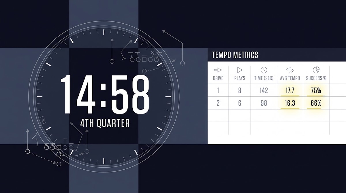
How Tempo Affects College Football Totals: A Practitioner’s Guide

How Tempo Affects College Football Totals: definition and context

How Tempo Affects College Football Totals starts with a simple premise: the pace of play defines the number of opportunities to score, so tempo must be a primary input when projecting game totals. Definitions matter because tempo is not a vague idea but rests on measurable statistics, notably plays, possessions or drives, and time of possession as defined for statisticians in college football 2024 NCAA Statisticians' Manual.

In applied work, analysts convert those core stats into operational tempo metrics such as seconds per play, plays per game, and possessions per game. Seconds per play especially provides a direct link from clock time to expected play counts by showing how long, on average, the game clock advances between snaps.

Seconds per play especially provides a direct link from clock time to expected play counts by showing how long, on average, the game clock advances between snaps.

Using tempo this way gives a structured way to separate available opportunities from scoring efficiency. That separation is useful: teams with similar points per game can produce different totals expectations if one side runs many more plays than the other.

How Tempo Affects College Football Totals: the core tempo metrics you must track

Seconds per play is computed by dividing a team or game clocked seconds of play by the number of plays, giving an average time between snaps; this metric is a practical bridge to plays-per-minute and total plays in a game. Season-level seconds-per-play values are often reported on public pace dashboards and provide a first-pass pregame input TeamRankings pace data.

Plays per game and possessions per game are complementary. Where seconds per play tells you how quickly a team moves the clock, plays per game and possessions estimate the number of discrete opportunities to run an offense. Possessions are useful when teams differ in how often they stop the clock on first downs or when you need to model drives explicitly.

A short example makes these metrics tangible. If a team averages 24 seconds per play and you estimate 130 possessions total between opponents, converting the seconds-per-play into plays gives an order of magnitude for total plays in the game, which you then scale by points per play to reach an implied total.

How Tempo Affects College Football Totals: why the 2023 timing-rule changes matter for projections

The 2023 timing rule change, where the game clock runs on first downs outside the final two minutes of each half, has a directional effect on available snap counts and therefore tempo baselines. Because the rule changes how the clock behaves after first downs, analysts should treat post-2023 seasons as the appropriate baseline for modern tempo work NCAA timing rules announcement.

Mixing pre- and post-2023 seasons can bias trend analyses, since older seasons reflect a different clock environment and typically show higher play counts per game in comparable matchups. For reproducible models and backtests, restrict the baseline to seasons where timing rules share the same operational clock behavior.

For 2026 projections, the practical recommendation is clear: use post-2023 data as your baseline when estimating plays and possessions to avoid systematic bias from earlier clock regimes.

How Tempo Affects College Football Totals: data sources and reproducible toolkits

Start with rule and stat references for definitions and authoritative guidance. The NCAA Statisticians' Manual provides the official definitions of plays, drives, and time of possession that underpin tempo metrics 2024 NCAA Statisticians' Manual and the NCAA stats site NCAA FBS stats.

For ready-made, season-level tempo inputs, public pace dashboards like TeamRankings’ seconds-per-play tables are practical and updated sources you can use as pregame inputs TeamRankings pace data.

When you need reproducible, granular calculations, play-by-play toolkits enable transparent opponent adjustments and derived tempo metrics. Tools that provide play-level exports let you calculate plays per drive, seconds per play, and opponent-adjusted efficiency in a fully auditable way cfbfastR or cfbstats.

How Tempo Affects College Football Totals: a step-by-step framework to project totals using tempo and efficiency

Use a staged workflow: estimate possessions, convert possessions to expected plays via seconds per play, then apply efficiency metrics to convert plays into point expectations. This structured sequence keeps tempo and efficiency distinct and easier to debug in backtests College Football Pace Report 2024.

Step 1, estimate possessions. Use season medians or team-specific possessions per game as your starting point. Step 2, estimate expected plays by combining possessions with seconds-per-play to produce a plays estimate. Step 3, apply points-per-play to those plays to reach an implied total.

Funded Plays Challenges

Review FundedPlays Challenges

When you test the workflow, keep tempo inputs and efficiency inputs versioned separately so you can identify which component produces an edge in head-to-head comparisons with market lines. (see Funded Plays)

Estimating possessions and total plays: worked formulas and quick approximations

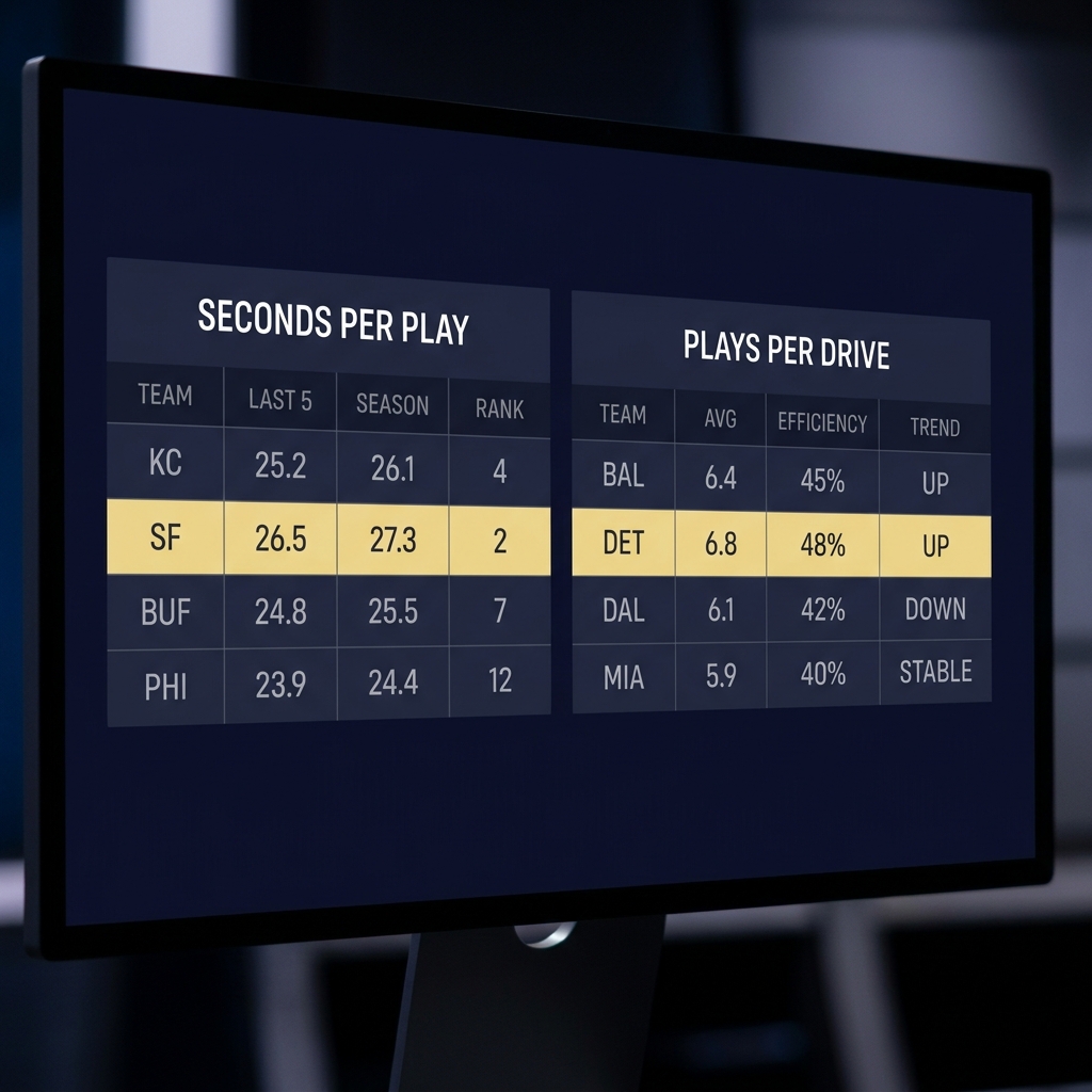
At its simplest, expected plays can be approximated with this formula: expected plays = game seconds divided by average seconds per play. For regulation college games, use 3600 game seconds as the baseline, then adjust for expected time lost to long clock stoppages or late-game strategy. Public seconds-per-play values make this conversion straightforward TeamRankings pace data.

If you prefer to start from possessions, use expected plays = estimated possessions per team times average plays per possession, where average plays per possession is available from play-by-play aggregations. When data are limited, substitute conference medians or opponent-adjusted seconds per play to avoid overfitting early-season samples cfbfastR.

Handle overtime by adding expected plays per overtime period based on league-standard formats, and for neutral-site games consider modest clock-management drifts if either team historically alters tempo away from home.

How Tempo Affects College Football Totals: applying efficiency - points per play and per drive adjustments

Efficiency is the multiplier that converts expected plays into expected points. Points per play (PPP) tends to be a more stable per-opportunity efficiency measure than raw points per game because it normalizes for pace and reduces variance from differing play counts College Football Pace Report 2024.

Compute offensive PPP by dividing season points scored by total offensive plays; compute defensive PPP similarly using points allowed. For an opponent-adjusted PPP, reweight those figures by opponent strength or use play-by-play based adjustments to remove schedule bias cfbfastR.

In practice, multiply the model’s expected plays by the combined PPP forecast to produce an implied total, then compare that result to the market number. Adjust for turnover-driven scoring variances conservatively, since turnovers can swing points without much change to tempo.

Opponent adjustments, game script, and situational modifiers

Adjust expected plays for an opponent’s pace rather than naively averaging two teams’ tempos; an effective approach is to compute a neutral plays baseline then apply opponent pace multipliers derived from play-by-play matchups. Public seconds-per-play and opponent-adjusted statistics are effective inputs for this adjustment TeamRankings pace data. (see how Funded Plays evaluations work)

Consider scenario-based modifiers. Blowouts typically reduce late-game plays as teams run the clock or substitute liberally, while close games often sustain or increase play counts. Treat these as conditional adjustments with conservative magnitudes and test them in backtests rather than assuming fixed values.

Non-tempo factors such as weather, key injuries, or coaching decisions should be folded in as additive modifiers to plays or efficiency. Make these adjustments explicit in your model so they can be measured for impact over time.

Decision criteria: when tempo-based signals should move your over/under lean

Use qualitative confidence bands and thresholds rather than single-number flips. For example, a large tempo plus efficiency gap that persists across several recent games and after opponent adjustments justifies a stronger lean than a single anomalous line. Tempo-driven edges should be weighted alongside injuries, weather, and market behavior College Football Pace Report 2024.

Combine signals by assigning repeatable weights: for instance, tempo model output 50 percent, market-mapping and residuals 30 percent, game-day intelligence 20 percent. Keep the weights consistent and document trades to understand whether tempo adds measurable edge.

Avoid overreacting to anomalies. Small-sample tempo shifts early in a season often revert; give these signals lower weight unless corroborated by opponent-adjusted evidence or a clear schematic change.

Common mistakes and pitfalls in tempo-based totals models

Mixing eras is a frequent error. Including pre-2023 seasons in a backtest when the timing rule changed introduces lookback bias and inflates historical play counts relative to the modern environment; use post-2023 seasons for contemporary baselines NCAA timing rules announcement.

Another common trap is using raw points-per-game without pace normalization. Teams that run fast will naturally score more points per game on average; points per play corrects for this by expressing scoring on a per-opportunity basis College Football Pace Report 2024.

Watch for statistical overfitting, lookahead bias in play-level adjustments, and failing to version opposing adjustments. Build simple holdout tests and prefer transparent, reproducible calculations from play-by-play sources.

Case studies: practical scenarios and example calculations using public pace data

Example 1: two fast-tempo teams. Inputs might be 22 seconds per play for Team A and 23 seconds per play for Team B, with combined possessions suggesting roughly 300 expected plays. Using a combined PPP of 0.35 produces an implied total near 105 points in raw arithmetic; the practical workflow refines that by opponent adjustments and turnover risk TeamRankings pace data.

Example 2: a fast offense versus a slow, clock-chewing defense. If Team A’s seconds per play indicate more snaps while Team B’s defensive scheme shortens possessions, the model should bias expected plays toward the faster pace but discount scoring efficiency where the defense limits big plays. Use play-by-play adjustments to capture those subtleties cfbfastR.

In both cases, compare the model’s implied total to the market line and document how much tempo and efficiency moved the projection. That record will show whether tempo adjustments consistently capture edges against live markets.

How to test, validate, and track a tempo-based totals model

Design backtests using only post-2023 seasons to ensure the evaluation environment matches the current clock regime. That approach prevents overstating model performance due to structural changes in how games are timed NCAA timing rules announcement.

Track metrics such as mean absolute error versus market totals, hit rate against market, and calibration plots that compare model-implied probabilities to observed frequencies. Version your code and inputs so you can reproduce results and isolate where improvements originate cfbfastR.

Iterate conservatively. When a new decision rule appears to add value, test it in a holdout and then in limited live samples before expanding its weight in the composite model.

How Tempo Affects College Football Totals: conclusion and practical next steps

This guide restates the workflow: use post-2023 baselines, gather seconds-per-play and possessions inputs, convert to expected plays, and apply points-per-play to produce an implied total. Keep tempo and efficiency separate so you can measure each component’s contribution to prediction quality 2024 NCAA Statisticians' Manual.

Three immediate actions are practical: gather season pace data from public dashboards, run a one-game worked example using the staged workflow (see our blog blog), and set up a backtest using post-2023 seasons to track model calibration. Finally, monitor coaching and tactical trends that could shift tempo over time and treat those shifts as hypotheses to test rather than facts.

References

- https://ncaaorg.s3.amazonaws.com/stats/stats_manuals/Football/2024FB_Stats_Manual.pdf
- https://www.teamrankings.com/college-football/stat/seconds-per-play
- https://www.ncaa.org/news/2023/4/21/media-center-playing-rules-oversight-panel-approves-football-timing-rules-changes.aspx
- https://cfbfastr.sportsdataverse.org/
- https://www.actionnetwork.com/ncaaf/college-football-pace-report-2024
- https://www.fundedplays.com/challenges
- https://cfbstats.com/
- https://www.ncaa.com/stats/football/Fbs
- https://www.teamrankings.com/college-football/stat/seconds-per-play?date=2025-01-10
- https://www.fundedplays.com
- https://www.fundedplays.com/blogs/how-fundedplays-evaluations-work
- https://www.fundedplays.com/blogs