How Small Edges Compound Over Time: A Practical Guide for Sports Predictors

What compounding of small edges means: definition and context

Why multiplicative outcomes matter

Compounding here means that each sequential decision multiplies your current account rather than simply adding an independent gain, so a small positive expected edge repeated over many rounds can change a path substantially over time.

When outcomes multiply, the geometric mean of per‑round returns governs long‑run growth rather than the arithmetic mean, which is why volatility and variation matter as much as average edge when you plan for long horizons.

Foundational results in the probability literature formalize how, under the right assumptions, a strategy that maximizes expected log wealth will outperform other fixed strategies over long horizons, making multiplicative compounding the key mechanism behind steady, incremental advantage.

Geometric mean versus arithmetic mean

Think of arithmetic mean as the simple average you get by adding returns and dividing by the number of rounds, while the geometric mean measures the average multiplicative factor per round and directly links to ending wealth after many repetitions.

The difference is practical: two strategies with the same arithmetic average return can have very different geometric returns if one is more volatile, so focusing on multiplicative growth helps explain why consistent, small positive edges matter in the long run.

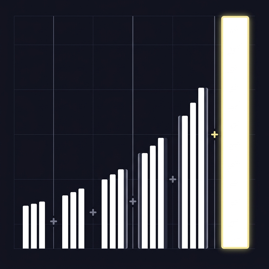
How Small Edges Compound Over Time

The phrase How Small Edges Compound Over Time captures the central idea for sports predictors: repeatable tiny advantages, when sized and managed correctly, can accumulate through multiplicative growth to meaningful long‑run improvement.

In the context of structured challenges and repeated predictions, this perspective emphasizes process, sizing discipline and measurement rather than one‑off wins.

How the math works: multiplicative returns and the driving formulas

Multiplicative model and log wealth

The basic mathematical insight is simple to state: if your wealth multiplies by a factor each round, the product of those factors over many rounds equals your final wealth, and taking logarithms turns that product into a sum that is easier to analyze.

Because logs convert products into sums, the average of log returns approximates the per‑round multiplicative growth rate and becomes the natural objective for long horizons, which is why maximizing expected log wealth is central to growth‑optimal sizing.

Formally, when opportunities repeat and independence assumptions hold, optimizing expected log wealth yields decisions that maximize asymptotic growth, a result that provides the mathematical justification for rules that focus on multiplicative performance.

Why log expectations matter for long horizons

The expected log return is directly tied to the geometric mean and to long‑run multipliers, so small increases in expected log can compound into large differences in terminal wealth over many rounds.

Because this metric penalizes variance, it balances average edge against volatility automatically, which explains why strategies that ignore multiplicative effects can overstate their long‑term prospects.

The Kelly criterion: a rules-based sizing framework

Origin and intuition

The Kelly criterion was derived in information theory and later formalized for favorable repeated gambles as the growth‑optimal sizing rule under specific assumptions; those derivations remain the foundation for sizing decisions that target long‑run growth.

The Kelly approach frames sizing as a direct tradeoff between edge and risk, seeking the fraction of capital that maximizes expected log wealth rather than short‑term wins.

Binary opportunity formula and interpretation

For a simple binary opportunity with win probability p and decimal payoff b, the classic Kelly fraction is f* = (b p − (1 − p)) / b, which gives a clear, rules‑based fraction to stake when the model assumptions are reasonable.

In that expression, the numerator measures the net expected gain per dollar risked and the denominator scales the fraction by the payoff, so the formula balances probability, payoff and the underlying edge in a single rule.

That clean formula is why many practitioners use Kelly as a starting point for sizing, while recognizing that real trading and prediction environments often require conservative adjustments.

For the binary case the Kelly fraction gives an explicit algebraic expression that is simple to apply when the model assumptions are met.

Why volatility and the geometric mean reduce compounded growth

Volatility drag explained

Volatility drag refers to the gap between arithmetic average returns and geometric average returns; because variance reduces the geometric mean, higher volatility erodes compounded growth even if the arithmetic mean looks attractive.

To appreciate the effect, imagine a strategy that alternates strong wins and losses: its arithmetic mean may be positive, but the multiplicative path can lose value because the losses have a disproportionate effect on the product of returns.

Implications for strategy performance

This means two strategies with the same expected payoff per round can produce very different long‑run outcomes depending on path volatility, which makes minimizing unnecessary variance an important complement to finding edges.

Investor education resources highlight compound interest and the role of variance when assessing long horizons, so translating arithmetic expectations into multiplicative outcomes is central to honest performance measurement.

Fractional Kelly and risk-constrained sizing: trading growth for stability

Why practitioners use fractional Kelly

Practitioners commonly use fractional Kelly, which scales the full Kelly fraction by a factor less than one, to reduce the risk of large drawdowns and to stabilize equity paths while retaining much of the long‑run growth potential.

Fractional sizing recognizes that estimation error and path dependence make the full Kelly fraction too aggressive for many real situations, offering a pragmatic compromise between peak growth and acceptable volatility.

Risk-constrained extensions and their goals

Research on risk‑constrained Kelly formulations adapts the growth‑optimal idea to include explicit limits on drawdown or tail risk, producing allocations that aim to preserve compounding benefits under additional safety constraints.

Those constrained variants are designed to change sizing outcomes in predictable ways so that a participant can control the tradeoff between peak long‑run growth and smoother, more resilient paths.

Practical limits: estimation error, correlation and changing payoffs

Edge estimation is noisy

Estimating small edges from historical data is inherently noisy, and this estimation error can substantially reduce the realized compounding benefit compared with an idealized Kelly plan that assumes perfect knowledge.

Because edge estimates can be biased or overfit to past samples, applying a full growth‑optimal fraction without accounting for uncertainty often leads to worse long‑run performance than a more cautious plan.

Correlation and dependence between opportunities

Correlation across opportunities and changing payoffs break the independence assumptions underlying classic growth‑optimal results, increasing the chance of clustered losses and larger drawdowns than predicted by simple models.

When predictions are correlated, aggregate volatility rises and realized geometric growth can fall well short of theoretical expectations, so practitioners must account for dependence when sizing or add explicit caps to limit aggregate exposure.

Funded Plays Challenges

Open a simulation spreadsheet

Skill-focused platforms that use virtual funded accounts can provide controlled environments to test sizing rules and record results without risking real capital, but users should still treat outcomes as indicative rather than guaranteed.

Decision criteria: when to use full Kelly, fractional Kelly or other rules

Personal risk tolerance and drawdown limits

Choose a sizing rule by mapping your tolerance for drawdown, confidence in edge estimates and required path stability to the known tradeoffs between a growth‑maximizing fraction and more conservative alternatives.

If you cannot accept large interim losses or your edge estimates are uncertain, fractional Kelly or explicit drawdown caps are generally more consistent with long‑term participation and survival.

Time horizon and evaluation structure

Short evaluation windows, strict drawdown requirements or platform rules that penalize early volatility favor conservative sizing, while long horizons and high confidence in independent edges create a stronger case for more aggressive fractions.

Whatever the choice, treat sizing as part of an adaptive process: monitor outcomes, update your edge estimates and adjust fractions to reflect changing information rather than locking a single rule indefinitely.

Typical mistakes and how to avoid them

Common behavioral and modeling errors

Common mistakes include overbetting above the theoretical optimum, ignoring correlation across opportunities and trusting noisy historical estimates as if they were exact; these errors cripple compounding by increasing drawdowns and shortening effective horizons.

Behavioral impulses to chase short‑term gains or to scale up after a winning streak directly oppose the discipline required to realize multiplicative growth over many rounds.

Practical fixes and safeguards

Practical safeguards include using fractional Kelly, setting conservative drawdown limits, validating edges out of sample and running paper simulations to see likely equity paths before committing to a sizing plan.

Regular recordkeeping that tracks geometric mean, rolling drawdown and realized variance helps spot model drift early and supports disciplined adjustment rather than reactive overleveraging.

Applying compounding principles to a sports prediction workflow

Integrating sizing into evaluation challenges

Translate the principles into a concise workflow: estimate your edge conservatively, choose an initial sizing rule such as fractional Kelly, simulate paths with your estimated distributions and set clear tolerances for drawdown and required geometric growth.

Document assumptions, preserve an audit trail of predictions and sizing choices, and design evaluation challenges so that results provide actionable signals about the robustness of your edge estimate.

Tracking performance and adapting over time

Track metrics that matter for compounding, chiefly geometric mean per round and maximum drawdown, and use those measures as primary signals to adjust sizing rather than focusing solely on cumulative wins or arithmetic averages.

Adaptive rules that modestly shrink sizing after periods of poor realized geometric returns, or that raise it when out‑of‑sample tests confirm edge persistence, provide a practical path to balance growth and survival over many repetitions.

Actionable checklist and closing summary

Key takeaways

Compounding of small edges works because multiplicative outcomes make expected log wealth the right long‑run objective, and growth‑optimal rules such as Kelly formalize how to convert an estimated edge into a sizing fraction.

Volatility reduces geometric growth relative to arithmetic expectations, so conservative adjustments like fractional Kelly and risk constraints preserve much of the compounding benefit while limiting damaging drawdowns.

Next steps for disciplined compounding

Checklist: estimate edges conservatively, run paper simulations, use fractional or constrained sizing, monitor geometric mean and drawdowns, and update sizing as evidence accumulates.

Remember that these tools do not guarantee outcomes; they provide a principled way to translate repeatable small advantages into disciplined long‑run progress when combined with honest edge estimation and consistent execution.