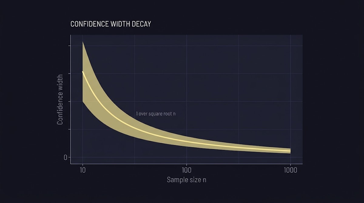
How Sample Size Affects Confidence: Practical Guide for Precision

How Sample Size Affects Confidence: definition and context

A confidence interval gives a range of plausible values for an unknown population quantity and the margin of error describes half that range for a chosen confidence level. Clear reporting of a point estimate together with its confidence interval and stated confidence level helps readers understand both the estimate and the uncertainty around it; official statistics guidance recommends reporting intervals alongside estimates to make uncertainty explicit Office for National Statistics guidance.

The basic idea behind How Sample Size Affects Confidence is intuitive: with more information about the population, estimates become more precise and the interval that expresses uncertainty gets narrower. The standard error measures how much a sample estimate typically varies from sample to sample, and standard statistical sources advise using confidence intervals and margins of error when presenting survey or study results U.S. Census Bureau margin of error guidance.

In this introductory section we use plain language, with one short numerical example to anchor the idea. Imagine a poll estimating the share supporting a proposal; a 500-person simple random sample will typically produce a wider margin of error than a 2,000-person sample because the standard error scales with sample size. Later sections show exactly how to compute those widths and plan sample size for a chosen margin of error.

What a confidence interval tells you

Think of a confidence interval as a statement about a procedure, not a single interval. Saying you have a 95 percent confidence interval means the method used will capture the true value in about 95 percent of repeated, hypothetical samples under the same design. The interval gives a plausible range and the margin of error gives a compact way to report how wide that range is. This interpretation and the practice of routinely reporting intervals is reinforced in methodological handbooks and official statistics guidance Cochrane Handbook guidance and in applied discussions such as Using the confidence interval confidently.

Why sample size enters the picture

Sample size enters through the standard error: larger samples reduce sampling variability and therefore shrink the standard error, holding population variability and confidence level fixed. In simple random sampling the algebra behind that relation leads directly to the familiar 1 over square root of n dependence that makes planning predictable. We walk through that algebra in the next section and show practical implications for planning.

The math behind it: why interval width scales with 1/√n

The formal reason that How Sample Size Affects Confidence follows a 1 over square root pattern is the behavior of the standard error. For a sample mean, the standard error equals the population standard deviation divided by the square root of the sample size. This relationship means the standard error is proportional to 1 divided by the square root of n; standard texts derive this result directly when they introduce sampling distributions OpenStax sample size and formulas.

To see why this matters for the interval width, recall that a two-sided confidence interval for a mean often takes the form point estimate plus or minus a critical value times the standard error. For large samples that critical value is a z-score, while for small samples a t critical value is appropriate; either way the margin of error is the critical value multiplied by the standard error. Because the standard error scales as 1 over the square root of n, the margin of error and thus the interval width do as well. The algebra is straightforward and leads to practical rules for how much precision improves when you increase n.

Derive the 1 over square root relationship for standard error

Write the standard error for a mean as sigma divided by the square root of n. The margin of error E is z times that standard error. Substituting shows E equals z times sigma over square root of n. Holding sigma and z fixed, E is proportional to 1 over square root of n. That proportionality is the backbone of the common heuristics researchers and practitioners use when designing studies.

One immediate practical implication follows algebraically: to halve E you must multiply n by four. That consequence is a direct result of the square root in the denominator and is commonly cited in planning guidance and textbooks as a rule of thumb for required increases in sample size.

Link between standard error and interval width

Because the margin of error is a product of a critical value and the standard error, anything that increases the critical value or the standard error widens the interval. In practice the critical value depends on the chosen confidence level and the standard error depends on sample size and population variability. That separation helps when planning: decide how much confidence you need, estimate variability, and pick a sample size that delivers the margin of error you want.

How Sample Size Affects Confidence: closed-form sample-size formulas

Closed-form formulas give quick, defensible answers for required sample sizes. For estimating a mean the usual approximate formula is n ≈ (z·σ/E)^2 where z is the critical value for your confidence level, sigma is an estimate of the population standard deviation, and E is the target margin of error. For a proportion the conservative planning formula is n ≈ z^2·p(1−p)/E^2, where p is the expected proportion; using p equals 0.5 yields the largest required n when no prior estimate is available NIST e-Handbook on confidence intervals.

These two formulas let you turn a desired margin of error and confidence level into a concrete sample-size target. In plain language: pick how precise you want to be, estimate how much variability you expect, choose a confidence level, and then compute n. The next paragraphs unpack the terms and show a tiny numeric illustration for each case so you can apply the formulas.

Formula for a mean: n ≈ (z·σ/E)^2

In the mean formula z is the critical z-score for the chosen confidence level, sigma is the standard deviation of the quantity of interest in the population or a reasonable proxy from pilot or past data, and E is the tolerable margin of error. Plugging these values into the formula and rounding up gives a sample size that achieves the targeted precision under simple random sampling assumptions. Open-access textbooks and methodological handbooks present this formula as the standard building block for precision planning OpenStax guidance.

Short numeric sketch: if you want E = 0.5 units with sigma ≈ 2 units and 95 percent confidence (z ≈ 1.96), then n ≈ (1.96*2/0.5)^2, which you compute and round up to the next whole observation. The method is straightforward to reproduce in a spreadsheet or calculator.

Formula for a proportion: n ≈ z^2·p(1−p)/E^2 and conservative p = 0.5

For a proportion p, the variance term is p(1−p) and it reaches its maximum at p = 0.5. Using p = 0.5 in the sample-size formula therefore yields a conservative, maximized required n when you lack a prior estimate. This conservative planning tactic is explicitly recommended in standard texts and handbooks to avoid underpowered sample sizes when prior information is weak OpenStax conservative p guidance.

When a prior estimate for p is available from pilot data or previous studies, using that value will usually lower the required n compared to the conservative choice; still, p = 0.5 is a safe default for early planning and communications with stakeholders.

When a prior estimate for p is available from pilot data or previous studies, using that value will usually lower the required n compared to the conservative choice; still, p = 0.5 is a safe default for early planning and communications with stakeholders.

How confidence level changes interval width

Higher confidence levels require larger critical values, which multiply the standard error and widen the interval. For example, moving from a 95 percent to a 99 percent confidence level increases the critical z and therefore increases the margin of error at the same sample size. Guidance for systematic reviews and general methodological practice emphasizes weighing the preference for higher confidence against the cost of wider intervals and larger required samples Cochrane Handbook on precision and confidence.

In planning terms this means confidence level is a choice with real consequences: if you need a higher confidence level, plan for either a larger margin of error or a bigger sample. Conversely, if sample size is strongly limited, a lower confidence level will buy you narrower intervals at the cost of less conservative coverage.

Critical values and their effect

Critical values come from either the normal distribution for large samples or the t distribution when sample sizes are small and the population variance is unknown. The t distribution has heavier tails at small n, which enlarges the critical value compared to the normal z and therefore widens the interval. This is an important nuance when designing small studies: the apparent cost of a desired confidence may be higher because of t-based adjustment.

Choosing a confidence level in practice

Common practice uses 95 percent confidence for general reporting, 90 percent when seeking narrower intervals for exploratory work, and 99 percent when a more conservative statement is needed. The choice should reflect the consequences of being wrong and stakeholder expectations; planners should document the trade-offs they considered when setting the level.

Rule of thumb and quick takeaways: the 1/√n implications

The central mnemonic: because standard error scales as 1 over the square root of n, halving the margin of error requires about four times the sample size. That rule helps stakeholders set realistic expectations about how much additional data will shrink uncertainty. Textbooks and method guides routinely present this relationship as a planning shortcut OpenStax rule of thumb and instructional material such as Pearson teaching resources.

Funded Plays Challenges

Run a quick sample-size check

A useful corollary is that doubling the sample size does not halve the margin of error; it reduces width by about 29 percent because the square root of two is about 1.414. That modest gain is often smaller than nontechnical audiences expect, so it is helpful to translate sample-size increases into percentage reduction in the margin of error when discussing design choices.

Keep the rule pragmatic: it is a guideline under simple random sampling and fixed variability. Design features like clustering, weighting, or high nonresponse can change the relation and typically require inflating the nominal n to achieve the same precision.

Halving error needs quadrupling n

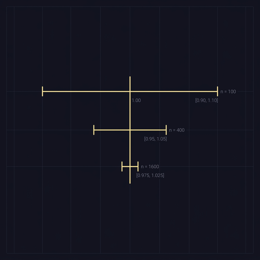
Algebraically, because E is proportional to 1 over the square root of n, setting E_new = E_old/2 implies sqrt(n_new) = 2 sqrt(n_old), so n_new = 4 n_old. This exact algebra explains the common instruction to quadruple the sample when seeking half the margin of error.

What doubling sample size actually buys you

Doubling n reduces the standard error by a factor of 1 over square root of two, which is about 0.707, so the margin of error falls by about 29 percent. That number is often surprising but can be computed quickly and communicated as part of design trade-offs with stakeholders.

Planning sample size step-by-step for common cases

Stepwise planning turns the formulas into an actionable workflow. The basic sequence is: define the acceptable margin of error E, choose a confidence level, estimate sigma or p from prior data or a pilot study (or choose conservative values), plug values into the appropriate formula, and round up the result. This structured approach is standard practice in methodological guidance and instructional materials NIST planning approach. See the Funded Plays homepage for practical posts on planning.

When estimating sigma, use a pilot study or historical data from a closely related context when possible. If only crude guidance exists, err on the side of larger variability to avoid underestimating the needed sample; similarly, use p = 0.5 for proportions when you lack a prior estimate to be conservative.

Stepwise checklist for means

1) State the target margin of error E in the units of the outcome. 2) Choose a confidence level and find the corresponding z or t critical value. 3) Obtain or estimate sigma from prior data or a pilot. 4) Compute n ≈ (z·σ/E)^2. 5) Round up and adjust for anticipated nonresponse or missing data by inflating n accordingly.

Practical note: if expected response rate is r, divide the computed n by r to plan how many contacts are needed to yield the target number of observations.

Stepwise checklist for proportions

1) Set the target margin of error E in proportion units. 2) Choose confidence level and z. 3) If you have no prior p, use 0.5 for planning; otherwise use the best available estimate. 4) Compute n ≈ z^2·p(1−p)/E^2. 5) Round up and inflate for design effects and nonresponse.

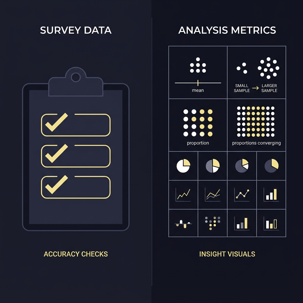
These steps translate easily into a spreadsheet where different values for p or sigma can be tested quickly to present scenarios for stakeholders.

Tools that help plan sample size and compute intervals

Several practical tools make planning and verification rapid: web-based sample-size calculators, spreadsheet templates that implement the closed-form formulas, and statistical software functions that compute exact intervals or sample-size requirements. These tools typically require the same inputs: desired margin of error, confidence level, and an estimate of variability or proportion. The U.S. Census and methodological handbooks recommend validating tool outputs against closed-form formulas for a quick sanity check U.S. Census Bureau guidance on margin of error. For practical examples and walkthroughs see the Funded Plays blog and tutorial modules such as the NHANES Reliability of Estimates module.

Before trusting tool output, check that the tool uses the same assumptions you intend: simple random sampling versus complex survey designs, normal approximation versus exact methods for proportions, and whether it accounts for finite population corrections if applicable. Simple spreadsheets often suffice, but verifying the underlying formula helps avoid silent misapplication.

When normal-approximation intervals mislead: small samples and extreme proportions

The usual large-sample approximations for proportions can mislead when sample sizes are small or the true proportion is near zero or one. In such settings the normal-based interval can undercover or produce bounds outside the feasible 0-to-1 range. Foundational literature recommends alternatives like the Wilson interval or exact Clopper-Pearson intervals for better coverage in these cases Statistical Science discussion of binomial intervals.

Practically, if your planned sample is small or you expect a rare event, choose software or formulas that implement Wilson or exact intervals rather than relying on the simple normal approximation. Doing so avoids systematic undercoverage and ensures reported intervals behave as intended.

Limits of the normal approximation for proportions

The normal approximation works well when np and n(1−p) are both reasonably large; when one of these products is small, the approximation degrades. That rule of thumb helps decide whether to use conservative sample-size planning or switch to alternative interval methods in the analysis stage.

Alternatives: Wilson and exact intervals

Wilson intervals adjust the center and width to improve coverage for small samples, and Clopper-Pearson exact intervals use the binomial distribution directly to produce guaranteed coverage at the cost of conservatism in some settings. Both options are well established and recommended in methodological literature where normal approximations fail.

Decision criteria: balancing precision, cost, and timeline

Setting a practical margin of error involves balancing the effect size you care about, the variability you expect, and the resources available. If a small difference matters to stakeholders, plan for a smaller E and therefore a larger n; if timelines or budget constrain sample collection, consider revising the confidence level or accepting wider intervals. Methodological guidance emphasizes aligning precision goals with operational constraints and documenting the rationale for chosen targets Cochrane Handbook on planning and precision.

Budget and time trade-offs can be explicit: compute sample sizes for multiple E values, present the costs of data collection for each scenario, and let stakeholders choose a level that matches risk tolerance and budget reality. In survey practice, it is common to show a small set of alternate plans to make the trade-offs concrete.

How to set a practical margin of error

Choose E based on what difference would change decisions or interpretations. In many applied contexts the margin of error should be smaller than the smallest effect size that matters in practice. Work with stakeholders to translate technical margins into business or policy-relevant terms.

Trade-offs when resources are limited

If resources constrain you, options include reducing the confidence level, accepting a larger E, improving measurement to reduce sigma, or using more efficient designs such as stratified sampling. Each choice has implications for interpretation and must be disclosed in reporting.

Common mistakes and how to avoid them

A frequent error is misapplying closed-form formulas without checking assumptions: ignoring clustering or weighting, failing to adjust for expected nonresponse, or using the normal approximation for small n or extreme p. These mistakes can produce intervals that are too narrow or misleading. The simple remedy is to check design assumptions, inflate n for design effects, and use exact or adjusted intervals when needed OpenStax cautions.

Another common oversight is reporting intervals without clearly stating the confidence level or the assumptions about the sampling process. Always state the confidence level, the sampling design, and any adjustments made for nonresponse or weighting in the methods section of a report.

Misusing formulas

Avoid plugging numbers into formulas blindly. Verify that sigma or p estimates come from a context similar to your planned study, and present sensitivity checks that show how required n changes with plausible variability values.

Ignoring design effects and nonresponse

When sampling is clustered or uses complex weights, the effective sample size is smaller than the nominal n. Plan to inflate nominal sample sizes by an estimated design effect and to increase contacts to compensate for expected nonresponse.

Practical examples: polls, A/B tests, and survey estimates

Example 1, a poll estimating a proportion: suppose you want a margin of error of plus or minus 3 percentage points at 95 percent confidence and you lack a prior estimate for p. Use p = 0.5, z ≈ 1.96, and E = 0.03 in the proportion formula to compute a conservative required n. This practical approach mirrors textbook examples and census-style planning when prior information is limited OpenStax polling example.

Example 2, an A/B test estimating a mean difference: estimate sigma from pilot results or historical experiments, decide the smallest detectable difference that matters, set E to half that difference if you want a two-sided interval around the difference, pick a confidence level, and use the mean formula to compute the needed per-group sample size. Reporting the resulting interval and the assumptions made is essential for interpretation. For an example of how we handle evaluations, see how Funded Plays evaluations work.

Worked calculation: how to change n to halve margin of error

Algebraic demonstration: start with E = z·sigma/sqrt(n). To get E/2 set z·sigma/sqrt(n_new) = z·sigma/(2 sqrt(n_old)). Solving gives sqrt(n_new) = 2 sqrt(n_old) and hence n_new = 4 n_old. This algebra is the direct source of the quadrupling rule used in planning and communication of trade-offs NIST algebraic demonstration.

Numeric sketch: if your current plan calls for 400 observations and you want half the margin of error, prepare for roughly 1,600 observations before rounding and adjusting for design effects or nonresponse. In practice you will round up and factor in anticipated response rates when turning required n into target contacts.

Step through the algebra and numeric example

Step 1: write E_old = z·sigma/sqrt(n_old). Step 2: set E_new = E_old/2. Step 3: substitute and solve for n_new to find n_new = 4 n_old. Step 4: apply any design or operational adjustments and round up. These steps are simple to automate in a spreadsheet to show scenarios quickly.

Show rounding and practical adjustments

Remember to round sample-size calculations up to whole observations and to add margin for anticipated nonresponse. If you expect a 60 percent response rate, divide the computed n by 0.6 to get the number of initial contacts to plan.

How to report confidence intervals and communicate uncertainty

Best practice is to present the point estimate, the confidence interval, and the confidence level together in a single statement. For example: "The estimated proportion is 42 percent, 95 percent confidence interval 38 to 46 percent." Official statistics guidance recommends this clear, complete format to help readers interpret the findings correctly ONS reporting guidance.

Avoid saying the interval contains the parameter with a certain probability about the single computed interval; instead focus on the long-run interpretation of the procedure and state assumptions about the sampling process. Keep language about uncertainty concrete and tied to the chosen confidence level.

Best practices for labeling and interpretation

Always report the confidence level, the margin of error if you prefer that compact format, and any assumptions about variance estimates or design effects. Use plain language to explain what the interval means for nontechnical audiences.

Avoiding common misstatements

Do not claim the interval gives the probability the true value lies within it for the specific computed interval. Instead explain that the method used has a certain coverage property across hypothetical repeated samples under the stated assumptions.

Conclusions and a quick checklist

Key takeaways: standard error scales with 1 over the square root of n so larger samples give narrower intervals; the closed-form formulas for means and proportions let you plan sample size for a target margin of error; use p = 0.5 for conservative planning when you lack a prior estimate; and switch to Wilson or exact intervals when small samples or extreme proportions make normal approximations unreliable Statistical Science on alternatives.

Quick planning checklist: 1) Define the margin of error you need. 2) Choose a confidence level. 3) Estimate sigma or p, using conservative defaults if necessary. 4) Compute n with closed-form formulas and round up. 5) Adjust for design effects and nonresponse and document assumptions. Use the checklist to guide transparent discussions with stakeholders and to produce reproducible plans.