How Game State Changes Fair Probability, and What to Do About It

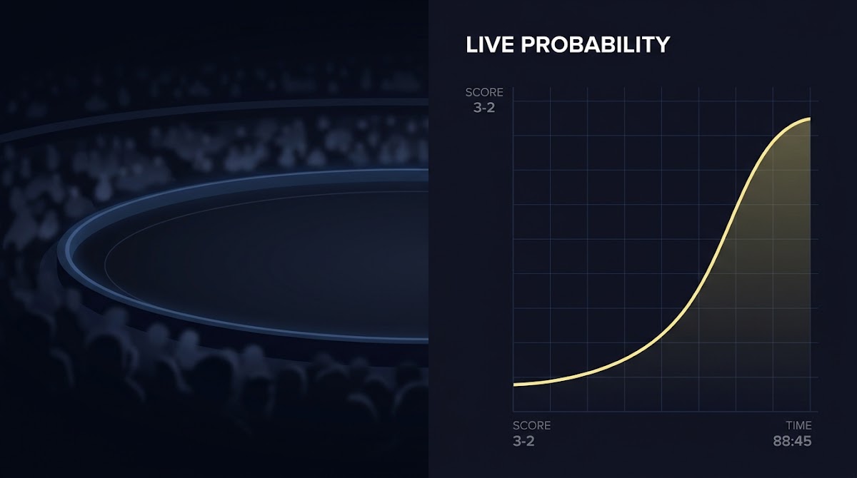
What fair probability means and why game state matters

Definition of fair probability in sports contexts, How Game State Changes Fair Probability

Fair probability is the best estimate of an outcome given the information available at a specific moment. It is not a gut feeling or a crowd opinion; it is the objective chance you would assign after accounting for known facts about the game state and valid statistical models.

Pregame probabilities come from projected strengths and season-long data. Those projections form a baseline. As the match unfolds, new, reliable information arrives and the baseline should be updated to produce a live fair probability that reflects the current context.

To make this practical, imagine a tied football game with three minutes left and your team on the opponent 10-yard line. That single fact changes the chance of winning compared with kickoff. The change is not magic; it reflects fewer remaining scoring opportunities, a specific possession advantage, and the scoreboard situation.

Fair probability is model-derived when possible. That means using a consistent method, whether simulation, empirical lookup, or statistical update, to translate game-state inputs into a percentage chance. Subjective belief can guide intuition, but disciplined updates should rely on documented rules or models rather than ad hoc reactions.

Overview of game state as a collection of variables

Game state is the set of variables that jointly determine remaining outcomes. Core variables are score margin, time remaining, possession or inning, player availability, and environmental factors such as wind or temperature. Each variable has a predictable direction of influence in most sports.

Score and time interact. A two-possession lead with ten minutes left is vastly different from the same lead with one minute left. Possession and field position change short-term expected scoring. Player availability or sudden substitutions can alter expected values for future plays. Finally, environmental changes like sudden rain can affect play styles and scoring rates.

Updating fair probability means integrating each reliable change, not every noisy fluctuation. The emphasis is on data quality and relevance. When new facts materially alter future scoring opportunities, models should reflect that change in the live probability estimate.

Score margin is often the single strongest driver of win probability. Every additional point the leading team holds reduces the trailing team’s remaining required scoring, but the practical effect depends on how many scoring chances remain. A three point lead in basketball with two minutes left is small; the same margin with thirty seconds left is large because the number of remaining possessions is limited.

How specific game-state variables shift fair probability

Score margin and leverage

Leverage refers to the value of each remaining scoring opportunity. When time is short, each possession carries higher leverage. That changes how the same scoring event moves fair probability: a turnover with two seconds left is worth more than one at halftime.

Time remaining and remaining opportunities

Time remaining sets the horizon for remaining events. More time generally makes outcomes more uncertain, because more scoring events can occur. Conversely, as the clock shrinks, probabilities compress toward the side favored by the current score, because there are fewer ways for the trailing side to recover.

Different sports schedule scoring frequency differently. Baseball has discrete innings with limited plate appearances per team. Basketball has many possessions and rapid scoring. The same time change has different quantitative effects across sports, but the qualitative rule holds: less time, fewer opportunities, and larger marginal impact for each event.

Possession, field position, and expected value

Who controls the ball and where matters because possessions translate to expected scoring. Field position converts into expected points or runs across the remaining plays. A team on the opponent 5-yard line has a much higher immediate expected value than the team backed up at its own 5.

Possession changes can flip short-term win probability a lot when the clock is limited. For longer horizons, possession matters less than cumulative expected scoring. This is why live models weight possession heavily for short-term forecasts and integrate it into simulations for longer windows.

Translating game-state changes into live prediction models

Types of live models: simulation, Bayesian updates, and empirical lookup tables

Live probabilities are typically produced by one of three families of approaches. Monte Carlo simulation runs many hypothetical continuations from the current state to estimate the frequency of outcomes. Bayesian updating treats the pregame model as a prior and adjusts that prior with new evidence to form a posterior probability. Empirical lookup tables use historical data to map common game states to observed outcome frequencies.

Each approach has tradeoffs. Simulations are flexible and capture complex interactions but require computation. Bayesian updates can be efficient when you can express new evidence as a likelihood function. Empirical tables are fast but limited by the granularity and representativeness of historical states.

Data inputs and update frequency

Quality and latency of inputs determine how reliable live estimates are. A model that receives accurate play-by-play inputs with minimal delay can update frequently. If inputs are noisy or delayed, rapid updates create more noise than signal. Decide an appropriate update cadence based on input reliability and computational cost.

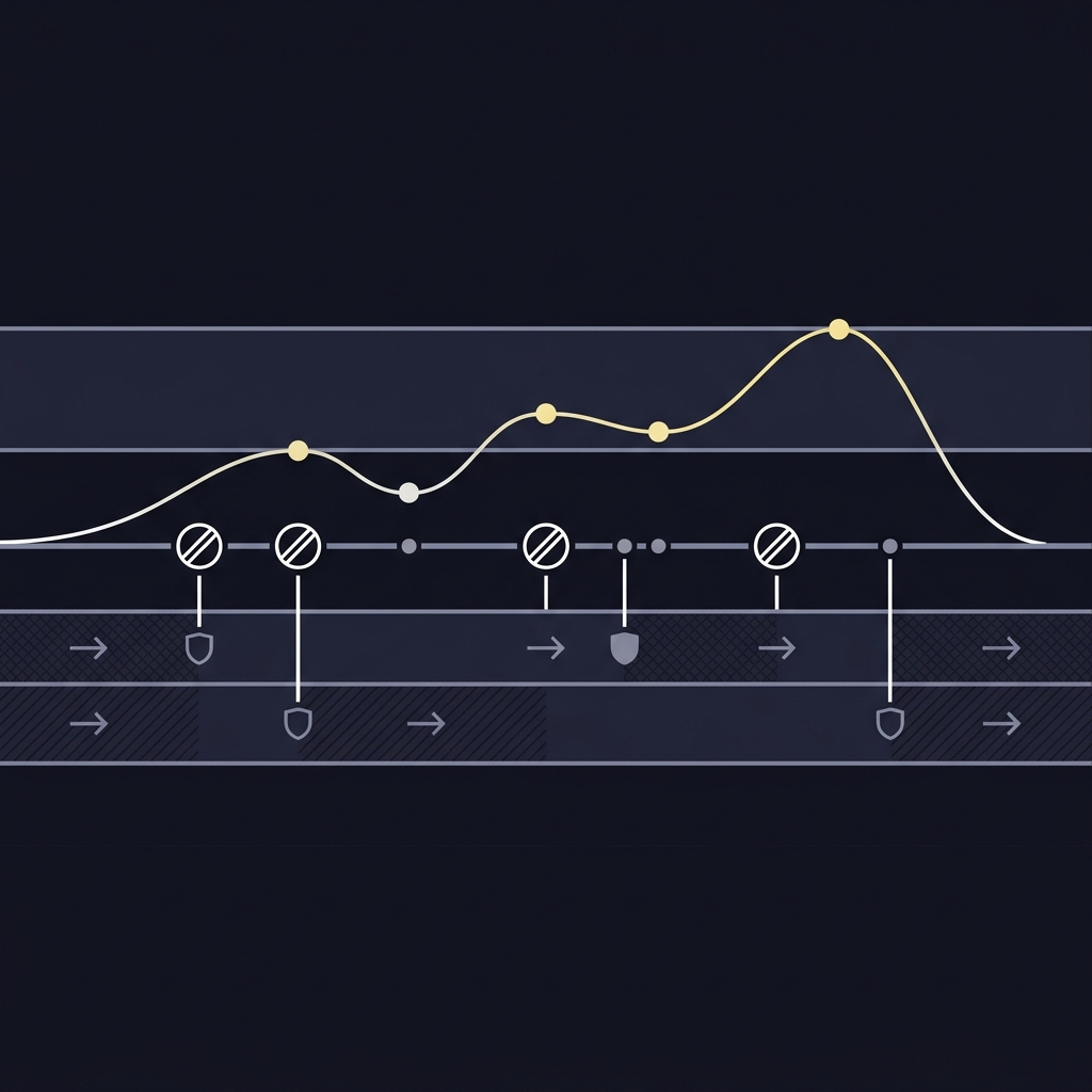
Sometimes a rules-based lookup or a small adjustment to a baseline probability is better than a costly full simulation. For example, when a likely scoring play has a predictable, narrow effect, a calibrated heuristic can capture the change with little computation. Use full recalculation when new information materially alters the state beyond simple heuristics.

Practical decision criteria: when and how much to update probability estimates

Thresholds for meaningful change

Not every change warrants a full probability recalculation. Use thresholds. Examples include a score change, a possession change in the final two minutes, a confirmed major injury, or a sudden weather shift that affects play. These thresholds keep updates meaningful rather than reactive to noise.

Another practical threshold is the expected change in outcome probability relative to your decision rule. If a new fact changes the predicted probability by less than a small percentage that would not change your selection or stake, skip the update until a larger signal appears.

Balancing noise and signal

Short-term events may reflect randomness rather than true shifts in underlying probability. A lucky bounce is often noise. To separate signal from noise, look for repeated or high-leverage events, corroborating data such as substitution patterns, or confirmed structural changes like a red card in soccer.

Documenting update rules helps: when you know what triggers an update, you avoid inconsistent judgments under pressure. Keep track of how often your rules would have fired historically to refine thresholds and improve calibration over time.

Common mistakes and pitfalls when shifting probabilities during a game

Overreacting to short-term momentum

Recency or momentum bias leads many decision makers to overweight a few recent plays. See Brian Burke's analysis on model usefulness.

When you upgrade a probability based on perceived momentum, ask if the change would have happened if the recent plays were replaced by average plays. If not, the momentum interpretation may be weak.

Ignoring structural constraints of the sport

Different sports have different structural limits on scoring opportunities. For example, once an inning ends in baseball certain scoring chances are gone until the next inning. In basketball, many possessions remain and a comeback is structurally more plausible. Models must respect those constraints to avoid implausible updates.

Other pitfalls include relying on delayed play-by-play input and making manual ad hoc edits that are not logged. Both can introduce model drift and break calibration. Maintain a clear audit trail of when and why you updated probabilities.

Step-by-step examples: updating probability in common sport scenarios

Example 1: late-game touchdown opportunity in football

Observable change: A team trailing by three has the ball at the opponent 8-yard line with 90 seconds remaining and all timeouts. Immediate decision: should you treat the trailing team as a favorite to win, and how much does the probability move?

Model adjustment logic: Short-term expected value is high for the trailing team because they have a clear scoring opportunity with multiple plays available. A rules-based approach might add a fixed uplift to the baseline win probability for possession inside the opponent 10 with under two minutes. A simulation would sample sequences of plays with clock management to estimate updated probability more precisely.

Example 2: extra-inning scoring chance in baseball

Observable change: Extra innings, runner on second, no outs. Immediate decision: how much does this single event move the chance of winning for the batting team?

Model adjustment logic: Baseball has discrete scoring sequences and small changes in run expectation can materially affect win probability. Here, the expected runs in the inning are higher than average. An empirical lookup or a situational run expectancy table captures the uplift quickly without a full simulation, which is appropriate when historical tables are well-populated.

Example 3: momentum swing in basketball

Observable change: A team goes on a 12-0 run and leads by eight with four minutes left. Immediate decision: does this run reflect a real shift in expected performance or just short-term variance?

Model adjustment logic: Evaluate supporting evidence. Are rotations different because a key defender was fouled out? Is the opponent missing players due to injury? If structural changes exist, increase the probability; if not, temper updates and favor calibration that recognizes high possession counts in basketball make short streaks less decisive than in low scoring sports.

Funded Plays Challenges

View challenges and templates

Using game-state aware probabilities in prediction challenges and bankroll management

How updated fair probability should inform staking and selection

Updated fair probability informs both selection and stake sizing. If a probability change moves a selection across your decision threshold, it may justify switching or hedging. For stake sizing, convert the updated probability into a recommended fraction of your risk budget using a disciplined rule such as a fixed fraction or Kelly-derived fraction sized to challenge limits.

Always cap exposure relative to drawdown limits. Consistency matters more in structured challenges than making occasional outsized bets. Documented rules for selection and stake sizing reduce emotional responses and help preserve long-term performance.

Responsible participation in skill-based challenge platforms

Platforms that use structured evaluation encourage consistent, repeatable forecasting. When you enter challenges, follow the published rules about position limits, drawdown thresholds, and eligible events. State-aware probabilities are valuable in these settings because they support disciplined decisions that align with challenge objectives.

FundedPlays is a skill-based sports prediction challenge platform where participants use structured, rule-based forecasting with virtual funded accounts to demonstrate consistency and qualify for performance-based rewards. Participation should be informed, disciplined, and compliant with each challenge's rules.

Measuring accuracy and calibrating live probability models

Key metrics: calibration, Brier score, and log loss

Calibration checks whether predicted probabilities match observed frequencies. If you predict 60 percent on many events, about 60 percent should happen. Scoring rules such as Brier score and log loss compare competing models without claiming one is perfect; they quantify the quality of probability forecasts. See recent work on the difficulty of estimating win probability.

Backtesting over many games is essential to see how a model performs across contexts. Watch for model drift when inputs or the sport itself changes. Regular monitoring helps identify when recalibration or new features are needed.

Backtesting and ongoing monitoring

Set up simple monitoring that records each update, the input state, and the eventual outcome. Aggregating performance over time reveals whether your update rules are well calibrated. If you find systematic over- or under-confidence, adjust model parameters or thresholds accordingly.

Conclusion: key takeaways and next steps for practicing game-state updates

Short checklist to apply before the next live event

Five quick steps: 1) Record the baseline pregame probability. 2) Define your update triggers. 3) Choose a simple heuristic for small changes and a full model for large changes. 4) Log every update and the reason. 5) Review outcomes and recalibrate. See more on the blog.

Developing discipline around updates improves long-term calibration. Keep your rules simple at first, then add complexity where it demonstrably improves accuracy. Responsible participation and clear documentation help you learn faster and maintain stable performance in challenge settings.