Building a Simple Sports Prediction Model: a practical guide

Introduction: why a simple probabilistic sports model matters

What this article will cover, Building a Simple Sports Prediction Model

A simple sports prediction model produces probabilistic forecasts for match outcomes rather than only class labels. Building a Simple Sports Prediction Model as a reproducible baseline helps you compare methods fairly, prioritize calibration, and run honest backtests before experimenting with more complex approaches. Reproducible baselines also make it easier to diagnose data leakage and to iterate on feature engineering without conflating changes in pipeline with changes in data splits, as described in standard model evaluation guidance scikit-learn model evaluation documentation.

This guide is aimed at practitioners who want a lightweight, runnable path from raw match records to logged per-event probabilities. It assumes familiarity with Python and basic machine learning concepts, but introduces time-aware validation and proper scoring in plain language. The roadmap covers: data and features, validation, model selection, probability calibration, rolling-window backtests, and simple serving options. See the Funded Plays blog for related posts.

Why evaluate probabilities with proper scoring rules

What are strictly proper scoring rules

When a model returns probabilities, we need metrics that reward honest probability estimates. Strictly proper scoring rules ensure that the expected score is optimized when the predicted probabilities match the true outcome probabilities; this property encourages calibrated forecasts rather than overconfident labels. The statistical foundations of strictly proper scoring are long established and remain central to evaluating probabilistic forecasts Journal of the Royal Statistical Society article on scoring rules.

Log Loss versus Brier score: when to prefer each

Two practical, commonly used proper scoring rules for binary outcomes are Log Loss and the Brier score. Log Loss (cross-entropy) strongly penalizes confident, wrong predictions and is appropriate when you care about sharp, well-separated probabilities. The Brier score measures mean squared error of probability forecasts and is easier to interpret on the same scale as probabilities. Both are useful diagnostics and choosing between them depends on whether you prefer sensitivity to extreme errors or a more directly interpretable squared-error view, as described in model evaluation guides scikit-learn model evaluation documentation.

The chosen metric affects model selection and calibration priorities: optimizing for Log Loss will favor models that avoid overconfidence, while Brier-focused workflows may emphasize reducing average squared error and improving calibration curves. Report both when possible to get a fuller view of performance.

Validation patterns for time-ordered sports data

Why standard cross-validation leaks information

Sports outcomes are ordered in time, and random k-fold cross-validation can mix future information into training folds, creating look-ahead bias. For example, if rolling averages or season-to-date features are computed before splitting, a random split can leak future match results into training and produce overly optimistic scores. Time-aware validation avoids this pitfall by preserving chronological order in training and test folds, which is critical for honest evaluation, as explained in modern time series cross-validation resources time series cross-validation guide and the scikit-learn cross-validation documentation.

Walk-forward backtesting and TimeSeriesSplit

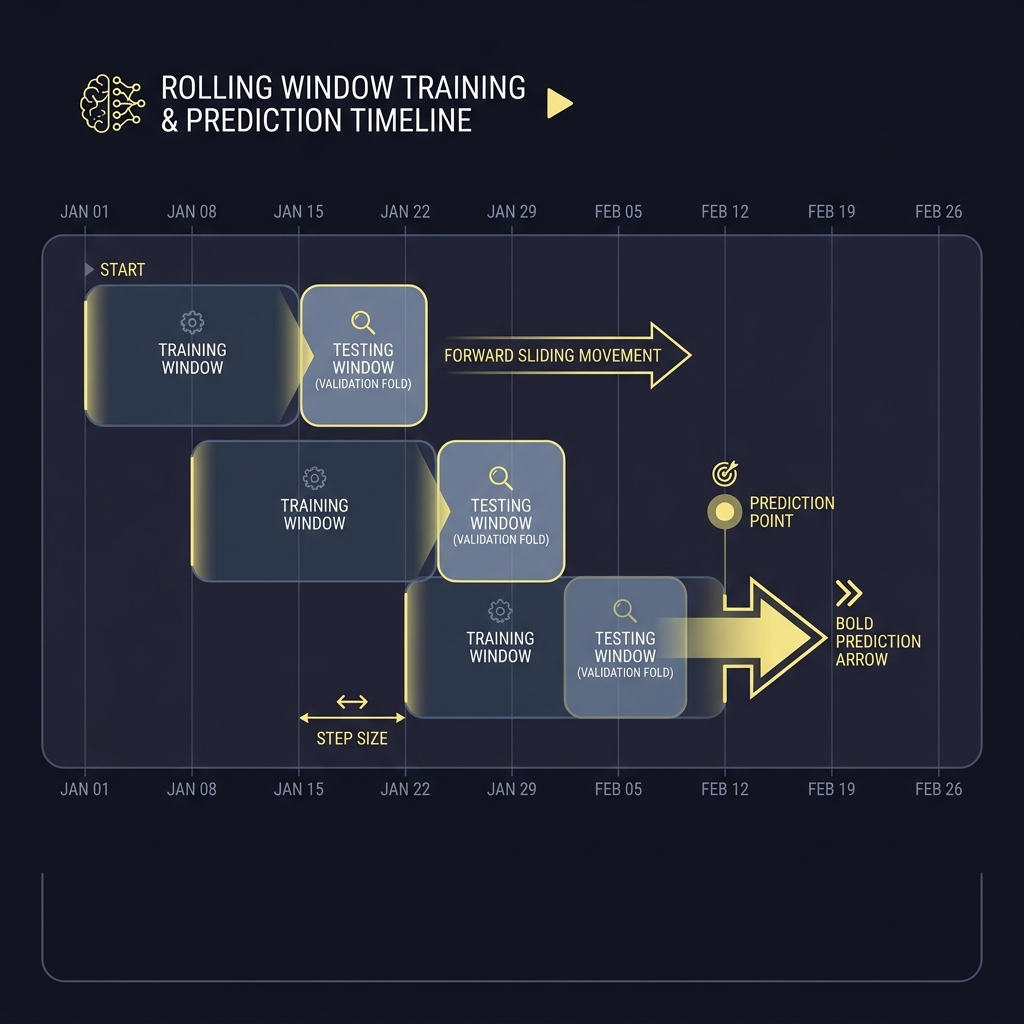
Walk-forward backtesting trains on an expanding window or sliding window of past matches and predicts a subsequent block of matches, then advances the window. A practical implementation uses TimeSeriesSplit or a manual rolling-window loop so that each prediction step only uses information available before the prediction date, which prevents leakage and better reflects real-world deployment scenarios time series cross-validation guide and a practical backtesting tutorial Machine Learning Mastery backtest guide.

Walk-forward backtesting trains on an expanding window or sliding window of past matches and predicts a subsequent block of matches, then advances the window. A practical implementation uses TimeSeriesSplit or a manual rolling-window loop so that each prediction step only uses information available before the prediction date, which prevents leakage and better reflects real-world deployment scenarios time series cross-validation guide.

Nested tuning to avoid optimistic bias

Hyperparameter tuning must also be time-aware. Use nested validation where the outer loop simulates chronological train versus test splits and the inner loop performs tuning only on past data within each outer train fold. This prevents information about the outer test periods from influencing hyperparameter selection and yields less biased performance estimates, consistent with best practices in model evaluation scikit-learn model evaluation documentation.

Data sources, features, and preprocessing

Common feature groups for win-probability models

Typical features include team strength proxies (season-to-date ratings or Elo-style scores), recent form measures (rolling averages over the last N matches), venue indicators (home, away, neutral), and matchup attributes such as rest days or travel. Choose features that can be computed only from past matches so they remain valid inside rolling-window backtests. When describing feature choices, reference how features will be computed and validated to make experiments reproducible scikit-learn model evaluation documentation.

Handling time, team-season identifiers, and missing data

Keep explicit identifiers such as team-season, matchdate, and match index. When building lag features or rolling statistics, assign them by chronological grouping so that every feature value uses only prior data. For missing values, prefer imputing with neutral or conservative defaults and add flags indicating imputation; this makes the model robust and the preprocessing auditable. Document these steps in the experiment artifacts so others can reproduce the pipeline.

Selecting a baseline classifier and hyperparameters

Why start with logistic regression

Logistic regression is a strong, interpretable baseline for binary outcome prediction and a sensible first step when Building a Simple Sports Prediction Model. It produces calibrated probability-like scores when regularized appropriately, is fast to train, and its coefficients are useful for sanity checks. The scikit-learn API keeps implementations consistent across preprocessing, cross-validation, and metrics, which helps maintain reproducibility scikit-learn model evaluation documentation.

Other lightweight baselines to consider

Consider simple alternatives for comparison: regularized linear models, small tree-based models, or an ensemble of simple learners. Keep hyperparameter grids small and focused to avoid long inner tuning loops in nested time-aware validation. Record seeds and package versions to ensure that runs can be reproduced and compared.

Funded Plays Challenges

Open FundedPlays Challenges page

Probability calibration and reliable outputs

Platt scaling and isotonic regression explained

Probability calibration corrects systematic miscalibration in classifier outputs. Platt scaling fits a sigmoid to map scores to probabilities, while isotonic regression fits a flexible non-decreasing mapping. Both methods are commonly used and remain effective for improving reliability of predicted probabilities when applied correctly on validation folds ICML paper on predicting good probabilities.

When to calibrate and how to evaluate calibration

Apply calibration using only out-of-sample validation data or through nested procedures so that calibration does not see the test fold. Evaluate calibration with a calibration curve or reliability diagram and measure change in Log Loss and Brier score to quantify improvement. Small visual checks and numeric comparisons help decide whether calibration materially improves decision-making.

Backtesting pipelines and rolling-window simulations

Designing a rolling window evaluation

Design a backtest that mirrors how predictions would be produced live: train on a past window, predict the next block of matches, store predictions, and advance the window. Decide on window size and step based on season structure and sample size; the rolling design avoids mixing future information into training and better approximates deployment conditions, a practice supported by time-aware validation resources time series cross-validation guide. For a concrete example of evaluation practices and how they are applied in competitions see how Funded Plays evaluations work.

Recording per-fold metrics and aggregating results

Log every per-event predicted probability and the true outcome so you can compute Log Loss and Brier score on a per-event basis and then aggregate. Report mean scores across folds and show variability across folds to avoid presenting a single overly optimistic number. Proper logging also helps debug data issues and supports reproducible reporting of results scikit-learn model evaluation documentation.

Simple deployment paths: serving a model for iteration

Lightweight options: REST API with FastAPI

For quick iteration, package the trained pipeline and expose a predict endpoint using a small REST service. A minimal FastAPI app that loads your serialized preprocessor and model can provide event-level probability predictions for dashboards or shadow deployments, which supports rapid experimentation and integration with monitoring systems FastAPI deployment documentation.

Model servers: MLflow and alternatives

If you need standardized model versioning and serving, methods like MLflow Models provide artifacts and serving options that simplify registry and A/B testing. Model servers can handle versioned artifacts and help standardize reproducible deployment practices, including packaging preprocessors and model code together MLflow model serving documentation.

Decision criteria: how to judge whether to trust model probabilities

Metric-based thresholds and calibration checks

Use combined signals to build trust: consistent improvement in proper scoring rules across chronological folds, calibration curve alignment, and low variance across folds are stronger indicators than a single good run. Prefer conservative acceptance criteria such as repeated improvement on Log Loss and Brier score across several rolling windows before trusting outputs for any operational decision, consistent with model evaluation guidance scikit-learn model evaluation documentation.

Operational considerations beyond accuracy

Also consider latency, explainability, and data availability. A slightly less accurate but interpretable and fast model may be preferable for exploratory dashboards or educational products. Document operational constraints alongside metric results so stakeholders understand trade-offs.

Common mistakes and how to avoid them

Typical leakage sources

Common leakage paths include using features computed with future outcomes, improperly computed rolling statistics that include the current event, and leaking season-level aggregates that span train and test splits. Check feature computation carefully and verify that every feature uses only past information to avoid optimistic evaluations, following time-aware validation best practices time series cross-validation guide.

Overfitting to short-term trends

Overfitting can occur when tuning intensely on a short period or when selecting features that capture transient noise. Mitigate this by re-running experiments with different seeds, shortening or lengthening windows, and holding out entire seasons where possible to ensure robustness across time scikit-learn model evaluation documentation.

Practical example: minimal scikit-learn pipeline for match probabilities

Dataset layout and feature table

A minimal dataset needs one row per match with columns for matchdate, home_team, away_team, outcome (binary for home win), and any precomputed features such as team rating, rolling form, and venue flag. Keep raw inputs and engineered features separate so you can reproduce feature computations during backtests and in deployment. Storing split indices and per-event metadata helps reproduce exact runs later scikit-learn model evaluation documentation.

Training loop with TimeSeriesSplit and calibration

Implement a training loop that uses TimeSeriesSplit or a manual rolling-window. For each fold: fit preprocessors and model on the training window, predict probabilities on the validation block, and optionally fit a calibration model on an inner validation split. Use CalibratedClassifierCV with time-aware inner folds or perform separate calibration fits per outer fold so calibration never sees the outer test data. Log per-event probabilities and compute Log Loss and Brier score for both uncalibrated and calibrated outputs to compare performance, following the calibration and evaluation practices described in ML literature ICML paper on predicting good probabilities.

Measuring impact and next steps after a baseline

From scores to decisions: what to track

Track both modeling metrics and operational metrics. Modeling metrics include Log Loss, Brier score, calibration diagnostics, and fold stability. Operational metrics include prediction latency, uptime, and ease of retraining. For experiment-driven improvements, pair metric tracking with clear decision rules for when a new model replaces an old one.

Small experiments to iterate safely

Use shadow deployments or A/B experiments to compare decisions driven by model probabilities against a control. Shadow deployments let you collect real-world data without changing behavior, and A/B tests can measure downstream impact if operational constraints permit. Always maintain reproducible backtests to justify any live changes.

Extensions and open methodological questions

Encoding domain priors and hierarchical effects

Advanced directions include incorporating team-strength priors, hierarchical models across leagues or seasons, and schedule effects. These extensions require careful, time-aware validation to ensure that added complexity genuinely improves out-of-sample probabilistic scores rather than simply fitting idiosyncrasies of the training period, as noted in forecasting discussions and statistical literature time series cross-validation guide.

Measuring value beyond accuracy

Measuring impact against market odds or user outcomes often demands custom metrics and experiment design. Consider how a model's calibrated probabilities change decision quality in your specific application and design experiments or business metrics that capture the value of improved probability estimates rather than raw accuracy alone.

Pre-release checklist: reproducibility, logging, and documentation

Artifacts to save and share

Save raw split indices, per-event prediction logs, trained model artifacts, and environment specifications. These artifacts let reviewers reproduce runs and verify claims. Prefer simple environment files and model serialization formats so experiments are portable and auditable, consistent with reproducible deployment advice FastAPI deployment documentation. Consider storing them on your project page at Funded Plays.

Minimum documentation for reproducible runs

Document the validation protocol, feature definitions, metric computations, and package versions. A short README that explains how to re-run the backtest and where to find logged predictions is often sufficient for others to verify and build on your baseline.

Conclusion: keep it simple, repeatable, and responsible

Time-aware validation, proper scoring rules, and probability calibration form the core of a responsible baseline workflow when Building a Simple Sports Prediction Model. Start with reproducible experiments, measure calibration alongside scoring, and prefer conservative acceptance criteria across multiple chronological folds.

Models do not guarantee outcomes. Use structured backtests and cautious deployment steps such as shadow runs and small experiments to evaluate real-world impact before changing production behavior.